Statistics 110 — Study Notes

Lecture-by-lecture study notes for Statistics 110, beginning with probability and counting.

Statistics 110: Probability, taught by Joe Blitzstein at Harvard University, introduces probability as a language for understanding uncertainty, randomness, and statistical reasoning. The course develops both intuition and mathematical problem-solving skills, beginning with counting and sample spaces before moving to conditional probability, Bayes’ rule, random variables, probability distributions, expectation, limit theorems, and Markov chains.

Follow the course video lectures on YouTube, or visit the official course website for supporting materials and practice problems.

Lecture 1 - Probability and Counting

Probability begins with a precise description of possible outcomes. For finite, equally likely outcomes, probability reduces to counting. The multiplication rule and combinations provide the tools to count poker hands and distinguish the four basic sampling cases.

Notation at a Glance

Symbol	Meaning
$S$	Sample space: all possible outcomes
$A\subseteq S$	Event: a subset of the sample space
$P(A)$	Probability of event $A$
$\lvert S\rvert$, $\lvert A\rvert$	Number of outcomes in the sample space and the event
$n!$	Factorial; $0!=1$
$\binom nk$	Number of unordered selections of $k$ distinct objects from $n$
$n$ and $k$	Number of available objects or types, and sample size
$A\cup B$, $A\cap B$, $A^c$	Union, intersection, and complement

Learning objectives

After studying these notes, you should be able to:

Define an experiment, an outcome, a sample space, and an event.
Explain when probability can be calculated by counting outcomes.
Apply the multiplication rule for counting.
Distinguish ordered selections from unordered selections.
Distinguish sampling with replacement from sampling without replacement.
Derive the combination formula and calculate the probability of a full house.
Explain your reasoning in words, including the assumptions behind your calculations.

Part 1 — Why probability matters

Probability provides a mathematical way to describe uncertainty. Applications of probability and statistics include physics, genetics, economics, game theory, finance, history, government, and everyday reasoning.

Historical example: Who wrote the disputed Federalist Papers?

Frederick Mosteller and David Wallace investigated whether Alexander Hamilton or James Madison wrote 12 disputed Federalist essays. They compared word frequencies in texts with known authorship, focusing on common words whose use is relatively stable across topics. These writing habits provided evidence for comparing the two possible authors using statistical methods, including Bayesian inference. Their analysis supported Madison as the author of all 12 disputed essays.

Core idea: Uncertainty can concern a fixed historical fact. The author does not change, but our assessment of who it was can change as we examine evidence. Probability provides a way to quantify that uncertainty and update it.

Historical example: Dividing the prize in an unfinished game

Games involving dice, coins, and cards have clearly defined outcomes, making them useful for developing probability models. In their 1654 correspondence, Pierre de Fermat and Blaise Pascal explored games of chance, including how to divide a prize fairly when a contest stops before either player wins. Their letters helped establish the foundations of modern probability.

For a simplified example, suppose Alice and Bob have equal chances of winning each independent round. The first to win three rounds receives a $100 prize, but play stops with Alice leading two wins to one. Alice needs one more win; Bob needs two.

Imagine two further rounds, including an unused round if Alice wins immediately. The four equally likely sequences of round winners are:

Next two round winners	Winner of the contest
Alice, Alice	Alice
Alice, Bob	Alice
Bob, Alice	Alice
Bob, Bob	Bob

Alice wins the contest in three of the four sequences, so her chance of winning is $3/4$; Bob’s is $1/4$. Dividing the prize in proportion to these chances gives Alice $75$ and Bob $25$.

Core idea: A fair division reflects each player’s chance of winning from the current position. Counting equally likely future sequences turns that idea into a precise calculation. The imagined unused round keeps all sequences the same length without changing the contest’s winner.

Main lesson: Intuition can be unreliable in probability. Precise definitions and explicit reasoning help us check it.

Part 2 — Experiments, sample spaces, and events

Experiment

Experiment Definition

An experiment is any process with possible outcomes whose result is not known in advance. It need not be a laboratory experiment.

Examples include tossing a coin twice, rolling two dice, or selecting five cards.

Outcome and sample space

An outcome is one possible result. The sample space, written as $S$, is the set of all possible outcomes.

For two coin tosses:

\[S=\{HH,HT,TH,TT\}.\]

The positions represent the first and second tosses, so $HT$ and $TH$ are different outcomes.

For two distinguishable six-sided dice:

\[S=\{(i,j):i,j\in\{1,2,3,4,5,6\}\}, \qquad \lvert S\rvert=6\times6=36.\]

Here, $\lvert S\rvert$ means the number of elements in $S$. You can distinguish the dice by color, or distinguish the first roll from the second.

Event

Event Definition

An event is a subset of the sample space:

\[A\subseteq S.\]

An event occurs when the observed outcome belongs to that subset.

For two coin tosses:

Event	Subset of the sample space
Both tosses are tails	$\{TT\}$
Exactly one head	$\{HT,TH\}$
At least one head	$\{HH,HT,TH\}$

Set notation refresher — supplementary

Unions, intersections, and complements translate statements about events into precise set notation:

Notation	Meaning
$A\cup B$	$A$ or $B$ occurs, including the possibility that both occur
$A\cap B$	Both $A$ and $B$ occur
$A^c$	$A$ does not occur; the outcomes in $S$ outside $A$
$\varnothing$	The empty event
$A\subseteq B$	Every outcome in $A$ also belongs to $B$

Part 3 — The naive definition of probability

For a finite sample space whose outcomes are equally likely:

\[\boxed{P(A)=\frac{\lvert A\rvert}{\lvert S\rvert} =\frac{\text{number of favorable outcomes}}{\text{number of possible outcomes}}.}\]

“Favorable” means that the outcome satisfies event $A$, whether or not that outcome is desirable.

The two essential conditions

The sample space is finite.
Its individual outcomes are equally likely.

Without these conditions, simply counting favorable and possible outcomes does not establish the probability.

Example: Two tails

If $HH,HT,TH,TT$ are equally likely, then:

\[P(\text{two tails})=\frac{1}{4}.\]

Only one of the four outcomes belongs to the event.

Fairness alone is not enough for a sequence

Equal chances of heads and tails on an individual toss do not, by themselves, guarantee that the four two-toss sequences are equally likely. Dependence between tosses can change their probabilities.

Supplementary illustration: Suppose the first toss is fair, but the second result always repeats the first. Each position individually has a 50% chance of heads, yet:

\[P(HH)=P(TT)=\frac12,\qquad P(HT)=P(TH)=0.\]

Independent fair tosses would make all four sequences equally likely. Independence is a concept developed more fully later in probability.

Two possibilities do not imply a 50–50 chance

Consider the claim: “There either is life on Neptune or there is not, so the probability of life is 1/2.” This argument is invalid because listing two possibilities does not establish that they are equally likely.

Key distinction: Not knowing the probability is different from knowing that outcomes are equally likely.

Intelligent life is a more restrictive condition than life of any kind. If $I$ is the event of intelligent life and $L$ is the event of any life, then:

\[I\subseteq L\quad\Longrightarrow\quad P(I)\le P(L).\]

Strict inequality requires positive probability for life without intelligent life; it does not follow from subset inclusion alone.

Another common trap — supplementary

For two fair, independent dice, the 36 ordered pairs are equally likely. The possible sums $2,3,\ldots,12$ are not equally likely.

There is one pair giving sum 2, but six pairs giving sum 7. Therefore:

\[P(\text{sum}=2)=\frac1{36},\qquad P(\text{sum}=7)=\frac6{36}.\]

Part 4 — The multiplication rule for counting

Suppose a process has $r$ stages. There are $n_1$ choices at stage 1, $n_2$ choices at stage 2 for each possible first choice, and so on. If stage $i$ always has $n_i$ choices after any allowed preceding history, then:

\[\boxed{\text{Number of complete outcomes}=n_1n_2\cdots n_r.}\]

Example: Ice cream

Ice cream choices Example

There are two cone types and three flavors available with either cone:

Choose a cone
├── Cake
│   ├── Chocolate
│   ├── Vanilla
│   └── Strawberry
└── Waffle
    ├── Chocolate
    ├── Vanilla
    └── Strawberry

Each complete path represents a different cone–flavor pair. There are:

\[2\times3=6\]

possible pairs. Choosing the flavor before the cone gives the same count: $3\times2=6$.

Why counting rules are useful

Ten stages with two choices each produce:

\[2^{10}=1024\]

outcomes. Listing every outcome quickly becomes impractical.

Clarifications — supplementary

This is a counting rule, not a claim about multiplying probabilities of independent events. Counting does not require a probability model.
The identities of available choices may change between branches, as long as the required number of choices at that stage stays the same.
If branches have different numbers of continuations, count the separate branches and add. For example, three flavors for cake cones and two for waffle cones give $3+2=5$ possibilities.

Part 5 — Factorials, ordered selections, and combinations

Factorial notation

For a positive integer $n$:

\[n!=n(n-1)(n-2)\cdots2\cdot1\]

For example, $4!=24$. The convention is $0!=1$.

Ordered selection without replacement

Select $k$ distinct objects from $n$, keeping track of selection order.

The first selection has $n$ possibilities.
The second has $n-1$ possibilities.
The third has $n-2$ possibilities.
The $k$th has $n-k+1$ possibilities.

The multiplication rule gives:

\[n(n-1)\cdots(n-k+1)=\frac{n!}{(n-k)!}.\]

Unordered selection without replacement

If order does not matter, the ordered count counts each group repeatedly. Every group of $k$ distinct objects has exactly $k!$ orderings.

Divide by that common overcounting factor:

\[\boxed{\binom nk=\frac{n!}{k!(n-k)!}.}\]

This is a binomial coefficient, read as “$n$ choose $k$.” It counts subsets of size $k$ from $n$ distinct objects.

For $0\le k\le n$, use the formula above. For nonnegative integers with $k>n$, the count is zero because the selection is impossible.

Small example — supplementary

Choose two people from $A,B,C$.

Ordered selections:

AB, BA, AC, CA, BC, CB

Unordered groups:

{A,B}, {A,C}, {B,C}

Thus:

\[\binom32=\frac{3\times2}{2!}=3.\]

Important: Division by $k!$ works here because every selected object is distinct and every group was counted exactly $k!$ times.

Counting full houses Worked example

Part 6 — Worked example: A full house in poker

Set up the model

A standard deck has 52 distinct cards: 13 ranks, each with four suits. A five-card hand is an unordered selection without replacement.

Assume every five-card hand is equally likely.

A full house contains exactly three cards of one rank and two cards of a different rank, such as three 7s and two 10s.

Step 1: Count all hands

\[\lvert S\rvert=\binom{52}{5}=2,598,960.\]

Step 2: Count full houses

Choice	Number of possibilities	Explanation
Rank of the three-card group	$13$	Any rank is possible
Three suits for that rank	$\binom43=4$	Choose three of its four cards
Rank of the two-card group	$12$	It must differ from the first rank
Two suits for that rank	$\binom42=6$	Choose two of its four cards

By the multiplication rule:

\[\lvert A\rvert=13\binom43\cdot12\binom42 =13\cdot4\cdot12\cdot6 =3744.\]

Each full house has a unique triple rank, pair rank, and selection of suits. The procedure therefore counts every full house exactly once.

Step 3: Divide

\[\boxed{ P(\text{full house})= \frac{13\binom43\cdot12\binom42}{\binom{52}{5}} =\frac{3744}{2,598,960} \approx0.001440576. }\]

That is approximately 0.1441%, or about one in 694 uniformly random five-card hands.

Common mistakes

Using 13 choices for the pair rank: Only 12 remain after choosing the triple rank.
Dividing the numerator by $2!$: The two ranks have different roles, so swapping them changes the hand’s rank multiplicities.
Using only $\binom{13}{2}$ for the ranks: After choosing two ranks, you must also choose which supplies the triple. An equivalent rank count is $\binom{13}{2}\times2=13\times12$.
Mixing an ordered denominator with an unordered numerator: Both counts must describe outcomes using the same convention.
Forgetting suits: Choosing ranks alone does not specify the actual five cards.

Part 7 — The sampling table

Two questions determine the basic counting method:

Does order matter? Would selecting $A$ then $B$ differ from selecting $B$ then $A$?
Is replacement allowed? Can the same object be selected again?

For $n$ distinct available objects or types and a sample of size $k$:

Sampling	Order matters	Order does not matter
With replacement	$n^k$	$\binom{n+k-1}{k}$
Without replacement	$\frac{n!}{(n-k)!}$	$\binom nk$

Assume $n\ge1$ and $k\ge0$. Without replacement, the displayed factorial expressions apply when $k\le n$; the count is zero if $k>n$.

With replacement, ordered

Each of the $k$ positions has $n$ choices:

\[n\times\cdots\times n=n^k.\]

Supplementary example: A four-digit code, allowing leading zeros and repeated digits, has $10^4=10,000$ possibilities.

Without replacement, ordered

Each selection removes an object:

\[n(n-1)\cdots(n-k+1)\]

Supplementary example: Awarding gold, silver, and bronze to three of eight people, with no ties, gives $8\times7\times6=336$ possibilities.

Without replacement, unordered

Select a group, ignoring order:

\[\binom nk.\]

Supplementary example: A three-person committee from eight people can be chosen in $\binom83=56$ ways.

With replacement, unordered

Repetitions are allowed, but order is ignored. Such a selection is called a multiset.

The number of such selections is:

\[\binom{n+k-1}{k}.\]

A small case helps illustrate what the formula counts:

Supplementary small-case check: Choose two items from $A,B,C$, allowing repetition and ignoring order:

AA, AB, AC, BB, BC, CC

There are six possibilities, agreeing with $\binom{3+2-1}{2}=\binom42=6$.

Why you cannot simply divide $n^k$ by $k!$ — supplementary

With repetition, different unordered selections can have different numbers of ordered versions. For example, $AB$ corresponds to $AB$ and $BA$, but $AA$ has only one ordering.

There is no uniform $k!$ overcounting factor.

A probability warning — supplementary

The sampling table counts possibilities; it does not automatically make them equally likely.

For two independent uniform draws from $A,B,C$, there are nine equally likely ordered sequences. After ignoring order:

\[P(AA)=\frac19,\qquad P(\{A,B\})=\frac29.\]

Although there are six multisets, they are not equally likely under this sampling process. Consequently, dividing by six would give incorrect probabilities for this experiment.

Part 8 — Original practice questions

Try these before reading the answers.

Two independent fair coins are tossed. Write the sample space and find the probability of exactly one head.
A cafe offers four drinks and three pastries, with every pairing available. How many drink–pastry pairs can you choose?
How many five-character strings can be formed from $A,B,C,D$ if repetition is allowed?
How many ways can a president and secretary be selected from seven people if one person cannot hold both roles?
How many three-person committees can be selected from seven people?
A bag contains five distinct red balls and three distinct blue balls. Two balls are selected uniformly without replacement. What is the probability that both are red?
How many unordered selections of three items can be made from four types if repetition is allowed?
Explain why “it happens or it does not happen” does not establish a probability of $1/2$.
In the full-house calculation, explain why the two rank factors are 13 and 12, and why there is no division by 2.

Part 9 — Practice answers

1. Exactly one head

\[S=\{HH,HT,TH,TT\},\qquad A=\{HT,TH\}.\]

The four sequences are equally likely, so $P(A)=2/4=1/2$.

2. Cafe pairs

Each drink can be paired with any of three pastries, giving $4\times3=12$ pairs.

3. Strings with repetition

There are four choices for each of five positions, giving $4^5=1024$ strings.

4. Distinct officer roles

There are seven choices for president and six remaining choices for secretary, giving $7\times6=42$ assignments. The roles matter.

5. Committee

Order does not matter, so the count is:

\[\binom73=\frac{7\cdot6\cdot5}{3\cdot2\cdot1}=35.\]

6. Two red balls

All unordered pairs of distinct balls are equally likely under the stated sampling process. There are $\binom82$ total pairs and $\binom52$ red pairs:

\[P(\text{both red})=\frac{\binom52}{\binom82} =\frac{10}{28}=\frac5{14}.\]

7. Unordered selection with repetition

Use the formula for unordered selections with replacement:

\[\binom{4+3-1}{3}=\binom63=20.\]

This is a count, not a claim that those selections are equally likely under every drawing process.

8. Two possibilities

The possibilities must also be equally likely before favorable-outcome counting gives $1/2$. The number of labels alone supplies no evidence of equal likelihood.

9. Full-house ranks

Any of 13 ranks can supply the triple. The pair must use one of the other 12 ranks. There is no division by 2 because the triple and pair roles distinguish the two ranks; each full house is already counted once.

Part 10 — Quick revision sheet

Concept	Essential fact
Sample space	Set of possible outcomes, $S$
Event	Subset $A\subseteq S$
Naive probability	$P(A)=\lvert A\rvert/\lvert S\rvert$ for finite, equally likely outcomes
Multiplication rule	Multiply stage counts when each stage has the stated number of choices after every allowed history
Ordered, with replacement	$n^k$
Ordered, without replacement	$n!/(n-k)!$
Unordered, without replacement	$\binom nk$
Unordered, with replacement	$\binom{n+k-1}{k}$
Full house	$13\binom43\cdot12\binom42/\binom{52}{5}\approx0.1441\%$

Term Glossary

Sample space Definition

The set of all possible outcomes of the experiment.

Event Definition

A subset of the sample space; it occurs when the observed outcome belongs to that subset.

Equally likely outcomes Definition

Outcomes assigned the same probability by the model. This assumption must be justified before applying the counting ratio.

Multiplication rule Definition

A counting principle that multiplies the numbers of choices at successive stages, provided each stage has the stated count after every allowed preceding history.

Combination Definition

An unordered selection of distinct objects, counted by a binomial coefficient.

Replacement Definition

Returning a selected object to the available pool so that it can be selected again.

Multiset Definition

An unordered selection that permits repeated objects or types.

Full house Definition

A five-card hand with three cards of one rank and two cards of a different rank.

Statistics 110 Lecture 1 Probability Counting Combinations

Lecture 2 - Story Proofs and Axioms of Probability

Counting becomes easier when a problem is represented in a useful way. Labeling clarifies which outcomes are distinct; stars and bars turns repeated selections into arrangements of symbols; story proofs establish identities by counting the same collection in two ways. Probability axioms then extend the framework to unequal probabilities and infinite sample spaces.

Notation at a Glance

Symbol	Meaning
$n$	Number of available types or labeled boxes in a stars-and-bars problem
$k$	Number of selections or identical objects to distribute
$x_i$	Number of selections of type $i$, or occupancy of box $i$
$\binom{n+k-1}{k}$	Number of unordered selections with replacement
$m,n$	Sizes of two disjoint groups in Vandermonde’s identity
$j$	Number selected from the first group
$S$	Sample space
$P(A)$	Probability assigned to event $A$
$\varnothing$	Empty event
$A_i\cap A_j=\varnothing$	Events $A_i$ and $A_j$ are disjoint
$\bigcup_{j=1}^{\infty}A_j$	Event that at least one of the events $A_1,A_2,\ldots$ occurs

Learning objectives

After studying these notes, you should be able to:

Distinguish labeled objects from unordered summaries of those objects.
Explain when dividing by an overcounting factor is justified.
Derive the stars-and-bars formula using a reversible encoding.
Recognize equivalent problems involving repeated selections, box occupancies, and integer solutions.
Prove three binomial identities by interpreting both sides as counts.
Explain why a count of possible configurations does not specify their probabilities.
State the probability axioms and apply additivity to disjoint events.

Part 1 — Labeling and correcting overcounting

Objects can look identical and still represent different outcomes

Suppose a jar contains three red balls and one green ball, and each physical ball is equally likely to be drawn. Label them $R_1,R_2,R_3,G_1$. The sample space for one draw has four equally likely outcomes, so:

\[P(\text{red})=\frac34.\]

The color labels “red” and “green” describe only two possible observations, but those observations are not equally likely. Red combines three underlying outcomes, whereas green corresponds to one.

Core idea: Labels make the elementary outcomes explicit. Ignoring a distinction in the final observation does not erase its effect on probability.

Example: Splitting ten people into teams of four and six

Choose the four-person team. Everyone else belongs to the six-person team:

\[\binom{10}{4}=210.\]

Choosing the six-person team first gives the same partition, so:

\[\binom{10}{4}=\binom{10}{6}.\]

There is no division by two: each partition has exactly one four-person team, so choosing that team counts each partition once.

Two unnamed teams of five Worked example

Now split ten people into two five-person teams with no labels or different roles assigned to the teams.

Choosing five people gives $\binom{10}{5}$ possibilities, but it counts each partition twice. Selecting one team first or selecting its complement first produces the same pair of teams.

Therefore:

\[\boxed{\text{Number of partitions}=\frac12\binom{10}{5}=126.}\]

If the teams instead have distinct labels, such as Team A and Team B, assigning a group to Team A differs from assigning that group to Team B. The count is then $\binom{10}{5}=252$.

Core idea: Decide what makes two completed results different before correcting for overcounting. Equal-sized, unnamed teams can be exchanged without changing a partition; labeled teams cannot.

When can you divide? Divide by a number $c$ only after showing that every desired outcome was counted exactly $c$ times. A correction that varies from outcome to outcome cannot be applied as one common divisor.

Part 2 — Unordered sampling with replacement

Choose $k$ times from $n$ available types, allowing repetition and ignoring selection order. Assume $n\ge1$ and $k\ge0$.

Instead of recording a sequence, record how often each type was chosen:

\[(x_1,x_2,\ldots,x_n),\qquad x_i\ge0,\qquad x_1+\cdots+x_n=k.\]

The entries are nonnegative integers. For example, choosing types $A,A,C$ gives counts $(2,0,1)$ for types $A,B,C$. Sequences $AAC$, $ACA$, and $CAA$ all give the same count vector.

Three equivalent counting problems Interpretation

The following descriptions refer to the same collection of possibilities:

Description	What one outcome records
Unordered sampling with replacement	How many times each type was selected
Identical objects in labeled boxes	How many objects occupy each box
Nonnegative integer solutions	A vector $(x_1,\ldots,x_n)$ whose entries sum to $k$

Each type corresponds to a box, and each selection adds one identical tally mark to that box. The boxes remain distinct because they represent different types; the tally marks do not need identities because order is ignored.

Check simple cases

Case	Direct reasoning	Formula check
$k=0$	One empty selection	$\binom{n-1}{0}=1$
$k=1$	Choose any one of the $n$ types	$\binom n1=n$
$n=1$	Every selection is of the only type	$\binom kk=1$
$n=2$	The first count can be $0,1,\ldots,k$; the second is determined	$\binom{k+1}{k}=k+1$

These checks help interpret the formula. They do not replace a proof for arbitrary $n$ and $k$.

Part 3 — Stars and bars: deriving the formula

Stars-and-bars formula Theorem

The number of ways to distribute $k$ identical objects among $n$ labeled boxes, allowing empty boxes, is:

\[\boxed{\binom{n+k-1}{k}=\binom{n+k-1}{n-1}.}\]

Equivalently, this counts nonnegative integer solutions of $x_1+\cdots+x_n=k$ and unordered selections of size $k$ with replacement from $n$ types.

Step 1: Encode the box counts

Use a star * for each object and a bar | between neighboring boxes.

For four boxes containing $(3,0,2,1)$ objects, the encoding is:

Box 1   Box 2   Box 3   Box 4
  ***   |      |  **   |  *

Compact encoding: ***||**|*

There are six stars and three bars. The adjacent bars indicate an empty second box. A leading bar would indicate an empty first box, and a trailing bar would indicate an empty last box.

Visual example: From boxes to a symbol string

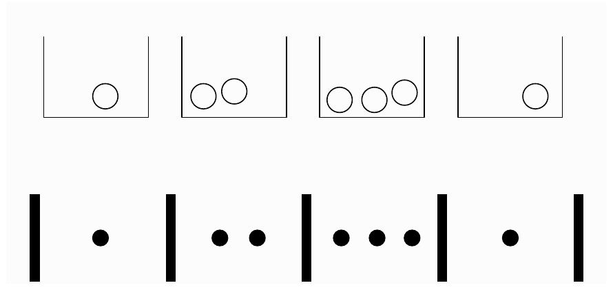
Four boxes containing one, two, three, and one particles, with the corresponding wall-and-particle encoding below. — Boxes and their symbol encoding. Reproduced from Joseph K. Blitzstein and Jessica Hwang, *Introduction to Probability*, Figure 1.5, p. 18.

The four boxes contain $(1,2,3,1)$ particles, so $n=4$ and $k=7$. Reading from left to right, each dot becomes a star and each boundary between boxes becomes a bar:

*|**|***|*

The lower row also shows an outer wall at each end. Those two walls are fixed; they are not extra separators to arrange. Removing them leaves seven stars and three internal bars, or ten positions. Thus all configurations of seven identical objects in four labeled boxes are counted by:

\[\binom{10}{7}=\binom{10}{3}=120.\]

Core idea: The box boundaries preserve the order of the labeled boxes, while the dots record only occupancies. The diagram uses seven particles; the earlier $(3,0,2,1)$ example uses six and shows how an empty box is encoded.

Step 2: Show that the encoding is reversible

Every occupancy vector produces exactly one string. Conversely, count the stars before the first bar, between successive bars, and after the last bar to recover every box count.

This is a bijection: a one-to-one correspondence between the two collections. Nothing is omitted and nothing is counted twice.

Step 3: Choose the star positions

A valid string contains:

$k$ stars;
$n-1$ bars;
$n+k-1$ positions altogether.

Choose which $k$ positions contain stars. All remaining positions contain bars:

\[\text{Number of strings}=\binom{n+k-1}{k}.\]

Choosing the $n-1$ bar positions instead gives $\binom{n+k-1}{n-1}$. Both descriptions specify the same strings.

For the example: Six objects among four boxes give $\binom96=\binom93=84$ possible occupancy vectors.

Why not choose gaps only between the stars? That would rule out adjacent bars and bars at the ends, excluding empty boxes. Stars and bars allows those arrangements because a type may be selected zero times.

Why not divide $n^k$ by $k!$? Different count vectors have different numbers of ordered versions. For example, $AAA$ has one ordering, while $AAB$ has three. There is no common $k!$ overcounting factor.

Supplementary example: Each box must be nonempty

Distribute seven identical objects into three labeled boxes, with at least one in each box.

First place one object in each box. Four objects remain, and they may be distributed with empty boxes allowed. Thus:

\[\binom{3+4-1}{4}=\binom64=15.\]

More generally, for $k\ge n\ge1$, positive integer solutions of $x_1+\cdots+x_n=k$ are counted by:

\[\binom{k-1}{n-1}.\]

If $k<n$, no such solution exists. The change of variables $y_i=x_i-1$ explains the result: the $y_i$ are nonnegative and sum to $k-n$.

Part 4 — A count is not a probability model

The stars-and-bars count is also called the Bose–Einstein value, reflecting its connection to counting occupation configurations of indistinguishable particles. For ordinary sampling problems, however, counting configurations does not establish that those configurations are equally likely.

Example: Two independent fair coin tosses

The four equally likely ordered outcomes are:

\[HH,\quad HT,\quad TH,\quad TT.\]

Ignoring order leaves three head–tail count configurations:

Configuration	Ordered outcomes represented	Probability
Two heads	$HH$	$1/4$
One head and one tail	$HT,TH$	$1/2$
Two tails	$TT$	$1/4$

Stars and bars correctly counts the three configurations:

\[\binom{2+2-1}{2}=3.\]

It does not imply that each has probability $1/3$. A model assigning equal probabilities to the three configurations would describe a different random experiment.

Core idea: Whether we can visually distinguish objects is separate from how the experiment assigns probabilities. Identical-looking coins still have a first and second toss, or can be labeled coin 1 and coin 2.

The physics connection has limits. Bose–Einstein counting concerns indistinguishable particles and their occupation configurations. It does not make ordinary coin-toss configurations uniformly distributed, nor does the counting formula alone determine a physical system’s probabilities.

Supplementary formula: Probability of a count vector

For $k$ independent draws, each uniformly choosing one of $n$ types, every ordered sequence has probability $1/n^k$.

A count vector $(x_1,\ldots,x_n)$ represents:

\[\frac{k!}{x_1!x_2!\cdots x_n!}\]

ordered sequences. To see why, arrange the $k$ selections and divide out the permutations within each repeated type. Therefore:

\[P(\text{counts }(x_1,\ldots,x_n)) =\frac{k!}{x_1!\cdots x_n!}\frac1{n^k}.\]

This explains precisely why different occupancy vectors generally receive different probabilities.

Part 5 — Story proofs: counting the same collection twice

Story proof Definition

A story proof establishes a mathematical result through an interpretation. For a counting identity, interpret both sides as the number of objects in the same collection, then justify each count.

A story proof is a general argument. Verifying a few numerical examples provides checks, but does not prove an identity for all admissible values.

Identity 1: Choosing a group or its complement

For integers $0\le k\le n$:

\[\boxed{\binom nk=\binom n{n-k}.}\]

Choose a committee of $k$ people from $n$ people. Specifying the members uniquely determines the $n-k$ nonmembers, and specifying the nonmembers uniquely determines the members.

The two sides count the same committees through complementary descriptions.

Core idea: Choosing what to include is equivalent to choosing what to exclude.

Identity 2: A committee with a president

For integers $1\le k\le n$:

\[\boxed{n\binom{n-1}{k-1}=k\binom nk.}\]

Count committees of size $k$ with one committee member designated as president.

Method	First choice	Second choice	Total
President first	One of $n$ people	Remaining $k-1$ members from the other $n-1$	$n\binom{n-1}{k-1}$
Committee first	A $k$-person committee from $n$	President from its $k$ members	$\binom nk\,k$

Every committee–president pair is counted exactly once by each method, proving the identity.

For example, selecting a three-person committee with a president from five people gives:

\[5\binom42=30=3\binom53.\]

Core idea: Changing the order in which we specify a complete outcome can produce a useful identity without changing the outcomes being counted.

Part 6 — Vandermonde’s identity

Vandermonde's identity Theorem

For nonnegative integers $m,n,k$ with $k\le m+n$:

\[\boxed{\binom{m+n}{k} =\sum_{j=0}^{k}\binom mj\binom n{k-j}.}\]

A binomial coefficient is zero when its lower argument exceeds its nonnegative upper argument. Impossible selections therefore contribute zero to the sum.

The story: Choose a committee from two groups

There are two disjoint groups: the first has $m$ people, and the second has $n$ people. Choose a committee of size $k$.

Count directly: Choose any $k$ of the total $m+n$ people:

\[\binom{m+n}{k}.\]

Count by composition: Suppose exactly $j$ committee members come from the first group. Then $k-j$ must come from the second group. For this fixed $j$, the multiplication rule gives:

\[\binom mj\binom n{k-j}.\]

Add over all possible $j$. The cases are disjoint because a committee has exactly one value of $j$, and they cover all committees. This proves the identity.

The feasible values are:

\[\max(0,k-n)\le j\le\min(k,m).\]

Using $j=0,\ldots,k$ is convenient because the infeasible terms are already zero.

Worked numerical example

Choose three people from a group of three and a separate group of four:

Number from the first group, $j$	Number from the second group	Number of committees
0	3	$\binom30\binom43=4$
1	2	$\binom31\binom42=18$
2	1	$\binom32\binom41=12$
3	0	$\binom33\binom40=1$

Hence:

\[4+18+12+1=35=\binom73.\]

Core idea: Multiply choices within a fixed case; add counts across disjoint cases.

Supplementary probability connection

If every $k$-person committee is equally likely, then:

\[P(\text{exactly }j\text{ from the first group}) =\frac{\binom mj\binom n{k-j}}{\binom{m+n}{k}}.\]

Vandermonde’s identity guarantees that these probabilities sum to 1. It connects a combinatorial identity to the requirement that all possible cases account for the whole experiment.

Part 7 — The general definition of probability

The formula $P(A)=\lvert A\rvert/\lvert S\rvert$ requires a finite sample space with equally likely outcomes. To handle unequal probabilities or infinitely many outcomes, assign probabilities to events through a function $P$.

Probability space Definition

At this introductory level, a probability space consists of:

A sample space $S$ describing possible outcomes.
A probability function $P$ that maps each event $A$ to a real number $P(A)$ in $[0,1]$ and satisfies the axioms below.

The input to $P$ is an event, which is a set of outcomes. Its output is a number.

Visual interpretation: Events are sets; probabilities are masses

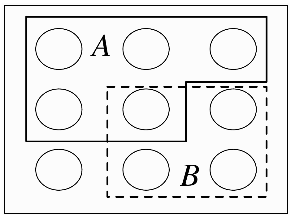
Nine outcomes represented by pebbles. Event A encloses five pebbles, event B encloses four, and one pebble belongs to both events. — Pebble World: each pebble is an outcome, and each outlined region is an event. Reproduced from Joseph K. Blitzstein and Jessica Hwang, *Introduction to Probability*, Figure 1.1, p. 3; the mass interpretation is developed in Section 1.6.

The outer rectangle is $S$. Event $A$ contains five of the nine outcomes; event $B$ contains four. One outcome belongs to both, so $A$ and $B$ are not disjoint.

If all nine outcomes are equally likely, each has probability $1/9$. Then:

\[P(A)=\frac59,\qquad P(B)=\frac49,\qquad P(A\cap B)=\frac19,\qquad P(A\cup B)=\frac89.\]

Adding $5/9$ and $4/9$ counts the shared pebble twice. Their union contains eight distinct pebbles, so direct addition is invalid here.

For a general finite model, imagine giving the pebbles nonnegative masses totaling 1. The probability of an event is the sum of the masses inside it. Equal masses recover counting; unequal masses require adding the assigned probabilities instead. The picture specifies which outcomes belong to each event, but the size or number of drawn circles alone does not specify their probabilities.

Core idea: Combining disjoint events adds separate masses. When events overlap, their common outcomes must be accounted for only once.

Axiom 1: The empty event and the whole space

\[\boxed{P(\varnothing)=0,\qquad P(S)=1.}\]

The empty event contains no outcome, so it cannot occur. The full sample space contains every possible outcome, so it must occur.

Axiom 2: Countable additivity

If $A_1,A_2,\ldots$ are pairwise disjoint events, then:

\[\boxed{P\left(\bigcup_{j=1}^{\infty}A_j\right) =\sum_{j=1}^{\infty}P(A_j).}\]

“Pairwise disjoint” means:

\[A_i\cap A_j=\varnothing\qquad\text{whenever }i\ne j.\]

No outcome belongs to two of the events. Their union therefore combines non-overlapping probability contributions.

Countable additivity also gives finite additivity: set all events after the last one to $\varnothing$. In particular, if $A\cap B=\varnothing$, then:

\[P(A\cup B)=P(A)+P(B).\]

Disjointness is essential. For two independent fair coin tosses, let $A$ mean the first toss is heads and $B$ mean the second toss is heads. The outcome $HH$ belongs to both events. Adding $P(A)+P(B)=1$ counts it twice, whereas $P(A\cup B)=3/4$.

Independent events are not necessarily disjoint. Independence describes how probabilities relate; disjointness means that the events cannot occur together.

Supplementary example: Unequal masses on a finite sample space

Let $S=\{a,b,c\}$, with individual probabilities $0.2,0.3,0.5$. For any event, add the probabilities of its outcomes. Then:

\[P(\{a,c\})=0.2+0.5=0.7.\]

The empty set has total probability 0, the full space has total probability 1, and disjoint sets add without double counting. This is a valid probability model, although counting two favorable outcomes out of three would give the wrong answer.

Equal masses of $1/N$ on a finite sample space of size $N$ recover the naive formula. Thus the counting definition is a special case of the general framework.

Supplementary example: A countably infinite sample space

Let $S=\{1,2,3,\ldots\}$ and assign:

\[P(\{j\})=2^{-j},\qquad j=1,2,\ldots.\]

The total probability is the geometric series:

\[\sum_{j=1}^{\infty}2^{-j}=1.\]

For example, the probability of an even result is:

\[P(\{2,4,6,\ldots\})=\sum_{r=1}^{\infty}4^{-r}=\frac13.\]

The outcomes are not equally likely, but the model has a well-defined total probability. No division by an infinite number of outcomes is needed.

Technical clarification for infinite spaces: In a fully general treatment, probabilities are assigned to a specified collection of measurable events, and a probability space is written $(S,\mathcal F,P)$. For finite or countable spaces, we can take all subsets as events. For uncountable spaces, such as a continuous interval, additional care is needed; not every subset must be assigned a probability.

Probability zero is not always impossibility. The empty event always has probability zero, but in continuous models a particular point can also have probability zero. The reverse implication is not generally valid.

Part 8 — Original practice questions

Try these before reading the answers.

How many ways can eight people be split into an unnamed team of three and a team of five? What changes for two unnamed teams of four? What if the two four-person teams are labeled A and B?
Encode $(2,0,1,2)$ using stars and bars. How many possible occupancy vectors are there for five identical objects in four labeled boxes?
How many nonnegative integer solutions satisfy $x_1+x_2+x_3=6$? How many satisfy the same equation with all entries positive?
Three independent draws select uniformly from types $A$ and $B$. How many unordered count configurations are possible? Find the probability of each configuration and explain why they are not uniform.
Prove $6\binom52=3\binom63$ by describing a committee and a president.
Choose three people from disjoint groups of four and five people. Use Vandermonde’s identity to verify the total count. If all committees are equally likely, what is the probability that exactly two members come from the first group?
Suppose $S=\{a,b,c\}$ has individual probabilities $0.1,0.4,0.5$. Let $A=\{a,b\}$ and $B=\{b,c\}$. Find $P(A)$, $P(B)$, and $P(A\cup B)$. Why is direct addition invalid?
In the model $P(\{j\})=2^{-j}$ for positive integers $j$, find the probability of a result at least 3.

Part 9 — Practice answers

1. Splitting teams

For teams of three and five, choose the three-person team:

\[\binom83=56.\]

For two unnamed teams of four, each partition is counted twice by selecting a four-person team:

\[\frac12\binom84=35.\]

For labeled teams A and B, choosing Team A uniquely determines Team B, giving $\binom84=70$ assignments.

2. Stars-and-bars encoding

The string is:

**||*|**

There are five stars and three bars, so:

\[\binom{4+5-1}{5}=\binom85=56.\]

3. Integer solutions

For nonnegative entries:

\[\binom{3+6-1}{6}=\binom82=28.\]

For positive entries, subtract one from each variable. The new nonnegative entries sum to 3, giving:

\[\binom{3+3-1}{3}=\binom52=10.\]

4. Counts versus probabilities

There are $\binom{2+3-1}{3}=4$ configurations. The eight ordered sequences are equally likely:

Counts $(x_A,x_B)$	Number of ordered sequences	Probability
$(3,0)$	1	$1/8$
$(2,1)$	3	$3/8$
$(1,2)$	3	$3/8$
$(0,3)$	1	$1/8$

The configurations are not uniform because they represent different numbers of equally likely ordered outcomes.

5. Committee and president

Choose the president from six people, then two other members from the remaining five: $6\binom52$.

Alternatively, choose three members from six, then select one of the three as president: $3\binom63$.

Both count the same committee–president pairs, and both equal 60.

6. Vandermonde and a committee probability

Count by the number selected from the first group:

\[\binom40\binom53+\binom41\binom52+ \binom42\binom51+\binom43\binom50 =10+40+30+4=84=\binom93.\]

Exactly two from the first group gives $\binom42\binom51=30$ committees, so:

\[P(\text{exactly two})=\frac{30}{84}=\frac5{14}.\]

7. Overlapping events

\[P(A)=0.1+0.4=0.5,\qquad P(B)=0.4+0.5=0.9.\]

Their union is $S$, so $P(A\cup B)=1$. Adding 0.5 and 0.9 counts outcome $b$ twice. Additivity in its direct form requires disjoint events.

8. An infinite tail

By countable additivity:

\[P(\{3,4,5,\ldots\})=\sum_{j=3}^{\infty}2^{-j} =\frac{1/8}{1-1/2}=\frac14.\]

Part 10 — Quick revision sheet

Concept	Essential fact
Labels	Identify elementary outcomes before grouping them into observations
Overcounting correction	Divide by $c$ only when every desired outcome is counted exactly $c$ times
Stars and bars	$k$ identical objects, $n$ labeled boxes, empty boxes allowed: $\binom{n+k-1}{k}$
Positive occupancies	For $k\ge n\ge1$: $\binom{k-1}{n-1}$
Complement identity	$\binom nk=\binom n{n-k}$
Committee–president identity	$n\binom{n-1}{k-1}=k\binom nk$
Vandermonde’s identity	$\binom{m+n}{k}=\sum_{j=0}^k\binom mj\binom n{k-j}$
Story proof	Justify two counts of the same collection
Probability function	Maps events to numbers in $[0,1]$
Normalization	$P(\varnothing)=0$ and $P(S)=1$
Countable additivity	For pairwise disjoint events, probability of the union equals the sum of probabilities
Main modeling warning	Equally likely sequences can produce unequally likely count configurations

Term Glossary

Occupancy vector Notation

A vector $(x_1,\ldots,x_n)$ recording the number of objects in each labeled box. For unordered repeated selections, it records how many times each type was chosen.

Bijection Definition

A one-to-one correspondence between two collections. Every element of either collection has exactly one partner in the other, so finite collections related by a bijection have the same size.

Stars and bars Counting method

An encoding of identical objects as stars and boundaries between labeled boxes as bars. Choosing the star or bar positions gives the number of nonnegative occupancy vectors.

Story proof Definition

A proof by interpretation. In combinatorics, it often establishes an identity by counting the same collection in two justified ways.

Vandermonde's identity Identity

An equality between choosing a committee from two combined groups and summing over all possible ways to split its membership between those groups.

Probability space Definition

A sample space together with a probability function on its events. In the fully general formulation, the collection of measurable events is also specified.

Pairwise disjoint events Definition

Events for which every pair of distinct events has empty intersection. At most one of them can occur in a single outcome.

Countable additivity Axiom

The probability of a union of countably many pairwise disjoint events equals the sum of their individual probabilities.

Statistics 110 Lecture 2 Stars and bars Story proofs Probability axioms

Lecture 3 - Birthday Problem and Properties of Probability

A coincidence can become likely when there are many opportunities for it to occur. The birthday problem illustrates this through counting the complement. Probability axioms give general rules for complements, containment, and overlapping events. Inclusion–exclusion then handles the overlaps in a shuffled deck, giving a surprisingly stable probability of at least one matching card.

Notation at a Glance

Symbol	Meaning
$k$	Number of people in the birthday problem
$M$, $M^c$	At least one birthday match, and no birthday matches
$\prod_{j=0}^{k-1}(1-j/365)$	Product of the $k$ factors for distinct birthdays
$A^c$	Complement of event $A$ within $S$
$B\cap A^c$	Outcomes in $B$ but outside $A$
$A\subseteq B$	Every outcome in $A$ belongs to $B$
$\bigcup_{i=1}^n A_i$	At least one of the events $A_1,\ldots,A_n$ occurs
$\bigcap_{i\in I}A_i$	All events whose indices belong to $I$ occur
$n$	Number of distinct cards in the matching problem
$\pi(i)$	Label on the card in position $i$ of a shuffled deck
$A_i=\{\pi(i)=i\}$	Card $i$ matches its position
$D_n$	Number of permutations of $n$ objects with no fixed points
$e$	Base of the natural logarithm; $e\approx2.71828$

Learning objectives

After studying these notes, you should be able to:

State the birthday model’s assumptions and identify its equally likely outcomes.
Derive the probability of at least one birthday match by counting the complement.
Distinguish any matching pair from a match with one specified person’s birthday.
Prove the complement rule, monotonicity, and the two-event addition rule from the probability axioms.
Explain the alternating signs in inclusion–exclusion.
Calculate intersection probabilities for specified matching positions in a permutation.
Derive the matching probability and explain its limit of $1-e^{-1}$.

Part 1 — The birthday problem: defining the model

Suppose $k$ people are in a room. What is the probability that at least two have the same birthday?

Use the following idealized model:

There are 365 possible birthdays; February 29 is excluded.
Each person’s birthday is equally likely to be any of those days.
People’s birthdays are mutually independent.
People are distinguishable: person 1’s birthday and person 2’s birthday occupy different positions in an outcome.

An outcome is an ordered list of $k$ birthdays. Each position has 365 possibilities, so:

\[\lvert S\rvert=365^k.\]

The uniformity and independence assumptions make every such list equally likely, with probability $365^{-k}$.

Let $M$ be the event of at least one match. A match may involve one pair, several pairs, or three or more people on one day. All of these belong to $M$.

Modeling clarification: Real birthdays need not be uniformly distributed or independent. The formula below is exact for the stated model; it is not an exact description of every real group. Labeling people does not establish independence—it specifies which outcomes we are counting.

Boundary cases

With zero or one person, a match is impossible. With more than 365 people, a match is certain by the pigeonhole principle: assigning more than 365 people to 365 days forces some day to receive at least two people.

With exactly 365 people, a match is extremely likely but not certain: an assignment with one person on each day is still possible.

Part 2 — Count no matches, then take the complement

Directly counting all possible kinds of matches is difficult because the cases overlap. The complement $M^c$ has a simple description: all birthdays are different.

For $1\le k\le365$:

Person	Allowed birthdays if all birthdays must differ
First	365
Second	364
Third	363
$k$th	$365-k+1$

Thus:

\[\lvert M^c\rvert=365\cdot364\cdots(365-k+1).\]

Divide by the number of equally likely birthday lists:

\[P(M^c)=\frac{365\cdot364\cdots(365-k+1)}{365^k} =\prod_{j=0}^{k-1}\left(1-\frac j{365}\right).\]

\[\boxed{P(M)=1-\prod_{j=0}^{k-1}\left(1-\frac j{365}\right),\qquad1\le k\le365.}\]

For $k=0$, the empty product is 1, giving probability 0. For $k>365$, use $P(M)=1$ rather than extending the product to negative factors.

Core idea: The experiment allows repeated birthdays, so the denominator counts sampling with replacement. The no-match event restricts birthdays to distinct days, so its numerator counts assignments without replacement. Both counts still describe ordered lists for the same labeled people.

Worked example: Why 23 people are enough

For 23 people:

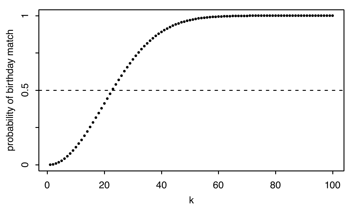
\[P(M)=1-\frac{365\cdot364\cdots343}{365^{23}} \approx0.507297.\]

The no-match probability is approximately $0.492703$. For 22 people, the match probability is approximately $0.475695$, so 23 is the smallest group size with a match probability above 50%.

People, $k$	Probability of at least one match
2	$0.002740$
10	$0.116948$
22	$0.475695$
23	$0.507297$
30	$0.706316$
50	$0.970374$
57	$0.990122$
100	$0.999999693$

Birthday-match probability rises with group size, crossing one half at 23 people and approaching one by 100 people. — Birthday-match probability under the independent, uniform 365-day model. Reproduced from Joseph K. Blitzstein and Jessica Hwang, *Introduction to Probability*, Figure 1.4, p. 12.

Why the result is less surprising after counting pairs

A group of 23 people contains:

\[\binom{23}{2}=253\]

pairs. The event concerns any of these pairs, not just the 22 comparisons involving one particular person. The number of pairs grows quadratically with group size.

Incorrect: There are 253 pairs, each matching with probability $1/365$, so the probability of a match is $253/365$.

Correction: Pair-match events overlap. If three people share a birthday, all three pairs among them match. Adding their probabilities counts that outcome repeatedly. The ratio $253/365\approx0.693151$ is not the probability of at least one match.

Supplementary comparison: Someone shares your birthday

Fix your birthday and consider 22 other people under the same independent, uniform model. Each avoids your birthday with probability $364/365$. Therefore:

\[P(\text{at least one shares your birthday}) =1-\left(\frac{364}{365}\right)^{22} \approx0.058571.\]

This is about 5.86%, compared with 50.73% for any match among all 23 people. The first event asks for a match with one specified birthday; the second allows any pair to match.

Part 3 — Probability axioms and the complement rule

A probability function assigns every event a number in $[0,1]$. The axioms are:

\[P(\varnothing)=0,\qquad P(S)=1,\]

and, for pairwise disjoint events:

\[P\left(\bigcup_{i=1}^{\infty}A_i\right) =\sum_{i=1}^{\infty}P(A_i).\]

These rules apply beyond finite, equally likely sample spaces. The following properties are consequences of the axioms, rather than additional assumptions.

Derive the complement rule

The events $A$ and $A^c$ are disjoint, and their union is $S$. By additivity:

\[1=P(S)=P(A\cup A^c)=P(A)+P(A^c).\]

Rearranging gives:

\[\boxed{P(A^c)=1-P(A).}\]

This justifies the final step in the birthday calculation. It also applies when individual outcomes have unequal probabilities or when the sample space is infinite.

Core idea: An event and its complement divide the entire experiment into two mutually exclusive possibilities, whose probabilities sum to 1.

Part 4 — Monotonicity: a larger event cannot be less likely

Monotonicity Theorem

If $A\subseteq B$, then:

\[\boxed{P(A)\le P(B).}\]

Proof by disjoint decomposition

Separate $B$ into the outcomes in $A$ and the outcomes outside $A$:

\[B=A\cup(B\cap A^c).\]

These two pieces are disjoint. Hence:

\[P(B)=P(A)+P(B\cap A^c)\ge P(A),\]

because probabilities are nonnegative.

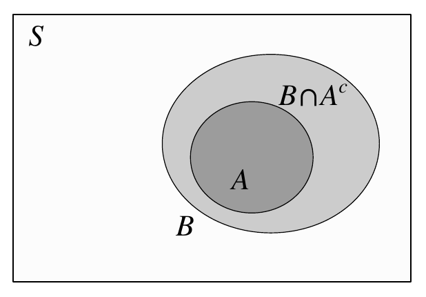
Event A lies inside event B; the remainder of B is labeled B intersection A complement. — Decomposing a containing event into disjoint pieces. Reproduced from Blitzstein and Hwang, *Introduction to Probability*, diagram in the proof of Theorem 1.6.2, p. 22.

Supplementary example: Nested dice events

Roll a fair six-sided die. Let $A=\{6\}$ and $B=\{4,5,6\}$. Since $A\subseteq B$:

\[P(A)=\frac16\le\frac36=P(B).\]

The extra outcomes $B\cap A^c=\{4,5\}$ contribute probability $2/6$.

Containment need not give strict inequality. Even if $A$ is a proper subset of $B$, it is possible that $P(A)=P(B)$. Strict inequality holds exactly when $P(B\cap A^c)>0$. A nonempty event need not have positive probability in every model.

Part 5 — Two overlapping events: the addition rule

For any two events $A$ and $B$:

\[\boxed{P(A\cup B)=P(A)+P(B)-P(A\cap B).}\]

The sum $P(A)+P(B)$ counts outcomes in the intersection twice. Subtracting $P(A\cap B)$ leaves each outcome in the union counted once.

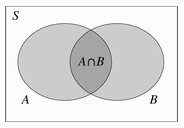
Two overlapping events A and B inside sample space S, with their shared region labeled A intersection B. — The intersection is included in both event probabilities. Reproduced from Blitzstein and Hwang, *Introduction to Probability*, diagram in the proof of Theorem 1.6.2, p. 22.

Proof using the axioms

Write the union as two disjoint pieces:

\[A\cup B=A\cup(B\cap A^c).\]

Therefore:

\[P(A\cup B)=P(A)+P(B\cap A^c).\]

Also, $B=(A\cap B)\cup(B\cap A^c)$ is a disjoint union, so:

\[P(B\cap A^c)=P(B)-P(A\cap B).\]

Substitution gives the addition rule. No independence assumption is needed. For disjoint events, the intersection has probability zero and the rule reduces to direct addition.

Supplementary worked example: An even result or a result above 3

For a fair die, let $A=\{2,4,6\}$ and $B=\{4,5,6\}$. Their intersection is $\{4,6\}$. Hence:

\[P(A\cup B)=\frac36+\frac36-\frac26=\frac46=\frac23.\]

The union is $\{2,4,5,6\}$, confirming the result by direct counting.

Core idea: “Or” includes outcomes where both events occur, but each such outcome contributes only once to the union.

Part 6 — Inclusion–exclusion for three or more events

Three events

\[\boxed{\begin{aligned} P(A\cup B\cup C) ={}&P(A)+P(B)+P(C)\\ &-P(A\cap B)-P(A\cap C)-P(B\cap C)\\ &+P(A\cap B\cap C). \end{aligned}}\]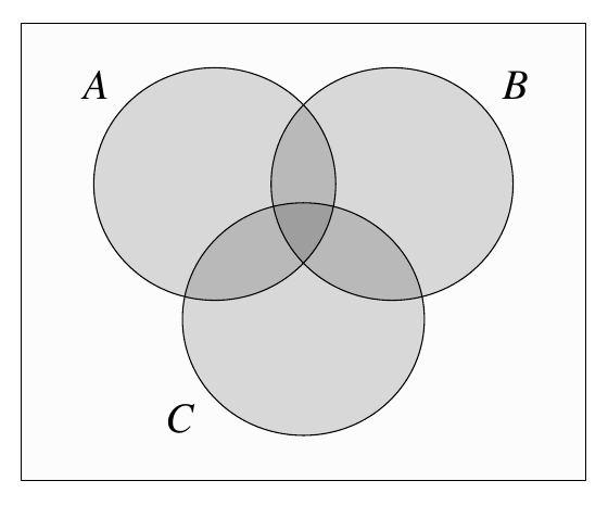

Three overlapping events A, B, and C, including pairwise overlaps and a central triple overlap. — Pairwise corrections remove the central overlap too many times, so the triple intersection is added back. Reproduced from Blitzstein and Hwang, *Introduction to Probability*, Section 1.6, p. 23.

Track how often a particular outcome contributes:

Events containing the outcome	Single-event additions	Pairwise subtractions	Triple addition	Net count
Exactly one	1	0	0	1
Exactly two	2	1	0	1
All three	3	3	1	1

The pairwise intersections include the triple intersection. Subtracting all three pairwise terms removes a central outcome three times after adding it three times, leaving zero. The final addition restores its contribution to one.

General formula

For events $A_1,\ldots,A_n$:

\[\boxed{ P\left(\bigcup_{i=1}^{n}A_i\right) =\sum_{r=1}^{n}(-1)^{r+1} \sum_{1\le i_1<\cdots<i_r\le n} P(A_{i_1}\cap\cdots\cap A_{i_r}). }\]

Add single-event probabilities, subtract two-event intersections, add three-event intersections, and continue with alternating signs. Each unordered group of indices appears once; the condition $i_1<\cdots<i_r$ prevents repeated listings of the same intersection.

Core idea: Inclusion–exclusion corrects overlap systematically. Symmetry makes it especially useful when all intersections involving the same number of specified events have the same probability.

Incorrect: For three events, subtracting the three pairwise intersections is enough.

Correction: The triple intersection must be added back. Pairwise intersections mean that both named events occur, whether or not a third event also occurs; they do not mean “exactly those two.”

Part 7 — de Montmort’s matching problem

Shuffle $n\ge1$ distinct cards labeled $1,2,\ldots,n$, with all $n!$ permutations equally likely. Reveal them in order while counting $1,2,\ldots,n$. Win if at least one revealed card matches the number called out.

A match is a fixed point of the permutation. If the deck is $(3,2,1,4)$, positions 2 and 4 match; positions 1 and 3 do not.

Let:

\[A_i=\{\pi(i)=i\}.\]

The event of winning is $A_1\cup\cdots\cup A_n$. The events overlap because several positions can match at once.

Step 1: One specified position matches

Fix card $i$ in position $i$. The remaining $n-1$ cards may be arranged freely, giving $(n-1)!$ favorable permutations:

\[P(A_i)=\frac{(n-1)!}{n!}=\frac1n.\]

Step 2: Several specified positions match

For distinct positions $i_1,\ldots,i_r$, fixing their cards leaves $(n-r)!$ arrangements:

\[P(A_{i_1}\cap\cdots\cap A_{i_r})=\frac{(n-r)!}{n!}.\]

For example:

\[P(A_i\cap A_j)=\frac1{n(n-1)},\qquad P(A_i\cap A_j\cap A_\ell)=\frac1{n(n-1)(n-2)}.\]

Fixing the specified positions does not forbid additional matches among the remaining positions. That is exactly what an intersection requires: all named events occur, possibly along with others.

Step 3: Group the inclusion–exclusion terms

There are $\binom nr$ ways to choose the $r$ specified matching positions. Each intersection has the same probability, so the total at order $r$ is:

\[\binom nr\frac{(n-r)!}{n!} =\frac{n!}{r!(n-r)!}\frac{(n-r)!}{n!} =\frac1{r!}.\]

Therefore:

\[\boxed{P(\text{at least one match}) =\sum_{r=1}^{n}\frac{(-1)^{r+1}}{r!} =1-\frac1{2!}+\frac1{3!}-\cdots+\frac{(-1)^{n+1}}{n!}.}\]

Core idea: A complicated union becomes manageable because intersection probabilities depend only on how many positions are specified. The binomial coefficient counts the choices of positions; the factorial ratio counts decks satisfying those choices.

Worked example: Three cards

For $n=3$:

\[P(\text{win})=1-\frac12+\frac16=\frac23.\]

All six decks can be listed:

Deck order	Matching positions	Result
$(1,2,3)$	1, 2, 3	Win
$(1,3,2)$	1	Win
$(2,1,3)$	3	Win
$(2,3,1)$	None	Lose
$(3,1,2)$	None	Lose
$(3,2,1)$	2	Win

Four of six permutations win. No permutation has exactly two matching positions: if two cards are fixed, the remaining card is forced into its own position.

Incorrect: Each position matches with probability $1/n$, so the probability of winning is $n(1/n)=1$.

Correction: The events are not disjoint. The fully ordered deck belongs to every $A_i$ and is counted $n$ times in that sum. Inclusion–exclusion corrects those repeated contributions.

Another trap: The match events are not independent. For $n\ge2$, $P(A_i\cap A_j)=1/[n(n-1)]$, whereas $P(A_i)P(A_j)=1/n^2$.

Part 8 — Derangements and the large-deck limit

A derangement is a permutation with no fixed points. It is a losing deck in the matching game.

Taking the complement of the winning probability gives:

\[P(\text{no matches})=\sum_{r=0}^{n}\frac{(-1)^r}{r!}.\]

Multiply by the total number of permutations:

\[\boxed{D_n=n!\sum_{r=0}^{n}\frac{(-1)^r}{r!}.}\]

For example, $D_3=6(1-1+1/2-1/6)=2$, agreeing with the two losing decks above.

The limiting probability

The exponential series gives:

\[e^{-1}=\sum_{r=0}^{\infty}\frac{(-1)^r}{r!}.\]

Consequently:

\[\boxed{P(\text{no matches})\longrightarrow e^{-1}\approx0.367879,}\] \[\boxed{P(\text{at least one match})\longrightarrow1-e^{-1}\approx0.632121.}\]

Cards, $n$	Exact winning probability	Decimal
1	$1$	$1.000000$
2	$1-1/2!$	$0.500000$
3	$1-1/2!+1/3!$	$0.666667$
4	$1-1/2!+1/3!-1/4!$	$0.625000$
5	$1-1/2!+1/3!-1/4!+1/5!$	$0.633333$
6	$1-1/2!+1/3!-1/4!+1/5!-1/6!$	$0.631944$

The finite probabilities alternate around the limit; they do not increase monotonically with deck size. A larger deck provides more candidate matching positions, but each specified position matches with smaller probability $1/n$.

Supplementary clarification: Accuracy of the limit

The alternating-series remainder bounds the error by the first omitted term:

\[\left|P(\text{win})-(1-e^{-1})\right|\le\frac1{(n+1)!}.\]

For six cards, the error is at most $1/7!\approx0.000198413$. For 52 distinct numbered cards, the limiting value is an extraordinarily accurate approximation, although the finite alternating sum remains the exact probability.

Part 9 — Original practice questions

Try these before reading the answers.

Under the birthday model, find the probability of at least one match among three people. Explain why there are two different counting rules in the calculation.
What is the smallest group size that guarantees a birthday match? Why does a group of 365 people not guarantee one?
Fix your birthday. Find the probability that at least one of ten other people shares it, under the independent, uniform model. Is this the same event as any birthday match among all eleven people?
Suppose $A\subseteq B$, $P(A)=0.25$, and $P(B)=0.60$. Find $P(B\cap A^c)$ and $P(B^c)$.
Suppose $P(A)=0.60$, $P(B)=0.50$, and $P(A\cap B)=0.20$. Find the probabilities of the union, neither event, and exactly one event.
Three events each have probability $0.40$. Each pairwise intersection has probability $0.15$, and the triple intersection has probability $0.05$. Find the probability of their union. What answer would omitting the triple correction give?
Shuffle five distinct numbered cards uniformly. Find the probability that positions 1 and 3 both match. How many permutations satisfy this condition? Does the condition forbid other matches?
For four distinct numbered cards, find the probability of winning the matching game and the number of derangements.
In a deck of four distinct numbered cards, explain why the probability that positions 1 and 2 both match is not $1/16$.

Part 10 — Practice answers

1. Three birthdays

The denominator counts all birthday assignments with repetition allowed. The no-match numerator counts only assignments of distinct birthdays:

\[P(M)=1-\frac{365\cdot364\cdot363}{365^3} =\frac{1093}{133225}\approx0.008204.\]

The probability is about 0.8204%. Taking the complement includes every possible kind of match without counting overlapping match cases separately.

2. A guaranteed match

The smallest size is 366. With 365 people, assigning exactly one person to each day produces no match. With 366 people, there are more people than available days, so at least two must share a day.

3. A specified birthday

All ten people avoid your birthday with probability $(364/365)^{10}$, so:

\[P(\text{at least one shares yours}) =1-\left(\frac{364}{365}\right)^{10} \approx0.027062.\]

This is about 2.7062%. Any match among eleven people also includes pairs among the other ten, so it is a different, larger event.

4. Containment and complement

The disjoint decomposition of $B$ gives:

\[P(B\cap A^c)=P(B)-P(A)=0.60-0.25=0.35.\]

The complement rule gives $P(B^c)=1-0.60=0.40$.

5. Union, neither, and exactly one

\[P(A\cup B)=0.60+0.50-0.20=0.90.\]

Neither event is the complement of the union, so its probability is $0.10$.

Exactly one consists of the disjoint events $A\cap B^c$ and $B\cap A^c$:

\[P(\text{exactly one})=(0.60-0.20)+(0.50-0.20)=0.70.\]

The union includes the both-events case; exactly one excludes it.

6. Three-event correction

\[P(A\cup B\cup C)=3(0.40)-3(0.15)+0.05=0.80.\]

Omitting the triple correction gives $0.75$, undercounting the union by the probability $0.05$ of the triple intersection.

7. Two specified matching positions

Fix cards 1 and 3 in positions 1 and 3. Arrange the remaining three cards in $3!=6$ ways. Thus:

\[P(A_1\cap A_3)=\frac{3!}{5!}=\frac1{20}.\]

Other positions may also match. The intersection requires at least the two specified matches, not exactly two matches.

8. Four-card game

\[P(\text{win})=1-\frac1{2!}+\frac1{3!}-\frac1{4!} =\frac{15}{24}=\frac58.\]

The no-match probability is $3/8$, so:

\[D_4=4!\cdot\frac38=9.\]

9. Dependence between matching positions

Each specified position matches with probability $1/4$. But fixing two specified cards leaves $2!$ favorable permutations out of $4!$:

\[P(A_1\cap A_2)=\frac{2!}{4!}=\frac1{12}.\]

Multiplying $1/4$ by $1/4$ would require independence, which does not hold for these events.

Part 11 — Quick revision sheet

Concept	Essential fact
Birthday sample space	$365^k$ equally likely ordered assignments under uniformity and mutual independence
No birthday match	$\prod_{j=0}^{k-1}(1-j/365)$ for $1\le k\le365$
At least one birthday match	One minus the no-match probability; exceeds 50% first at $k=23$
Guaranteed birthday match	$k>365$
Complement	$P(A^c)=1-P(A)$
Monotonicity	$A\subseteq B\Rightarrow P(A)\le P(B)$
Two-event addition	$P(A\cup B)=P(A)+P(B)-P(A\cap B)$
Inclusion–exclusion	Add singles, subtract pairs, add triples, and continue alternating
$r$ specified card matches	$(n-r)!/n!$
Total order-$r$ contribution	$\binom nr(n-r)!/n!=1/r!$
Matching-game win	$\sum_{r=1}^n(-1)^{r+1}/r!$
Derangements	$D_n=n!\sum_{r=0}^n(-1)^r/r!$
Large-deck win probability	$1-e^{-1}\approx0.632121$

Term Glossary

Birthday match Definition

An event in which at least two people share a birthday. It includes several pairs or larger groups sharing a day, not only exactly one matching pair.

Pigeonhole principle Counting principle

Placing more objects than boxes into boxes forces at least one box to contain two or more objects.

Complement rule Theorem

The probability that an event does not occur is one minus the probability that it occurs.

Monotonicity Theorem

If one event is contained in another, its probability cannot exceed that of the containing event.

Inclusion–exclusion Theorem

A formula for the probability of a union that corrects repeated contributions from overlapping events using alternating sums of intersection probabilities.

Permutation Definition

An ordering of distinct objects. There are $n!$ permutations of $n$ distinct objects.

Fixed point Definition

A position $i$ at which a permutation leaves the label unchanged: $\pi(i)=i$. In the matching game, it is a card whose label equals its position.

Derangement Definition

A permutation with no fixed points. In the matching game, it corresponds to a deck with no matching positions.

Statistics 110 Lecture 3 Birthday problem Probability properties Inclusion–exclusion Matching problem

Lecture 4 - Conditional Probability

Independence specifies when intersection probabilities can be multiplied. The Newton–Pepys problem combines independence, counting, and complements to compare three dice games. Conditional probability updates a probability when evidence is known: restrict attention to outcomes consistent with that evidence, then renormalize. Bayes’ rule relates the two directions of conditioning through the same joint probability.

Notation at a Glance

Symbol	Meaning
$A\cap B$	Both events $A$ and $B$ occur
$P(A\mid B)$	Probability of $A$ given that $B$ occurred; requires $P(B)>0$
$P(A\cap B)=P(A)P(B)$	Definition of independence of two events
$A^c$	Event that $A$ does not occur
$n$, $r$	Number of dice and number of sixes in a dice calculation
$\binom nr$	Number of choices of the $r$ dice that show six
$H$	A hypothesis whose probability is being updated
$E$	Observed evidence
$P(H)$	Prior probability of the hypothesis
$P(E\mid H)$	Likelihood: probability of the evidence if the hypothesis holds
$P(H\mid E)$	Posterior probability after conditioning on the evidence

Learning objectives

After studying these notes, you should be able to:

Use the mathematical definition of independence and distinguish it from disjointness.
Explain why independence also holds when either or both events are complemented.
Distinguish pairwise independence from mutual independence.
Count outcomes with exactly a specified number of sixes and solve the Newton–Pepys problem.
Interpret conditional probability as restriction and renormalization.
Calculate conditional probabilities with the correct conditioning event in the denominator.
Derive the multiplication rule for probabilities and Bayes’ rule.
Distinguish a likelihood from a posterior probability and explain why reversing the conditioning bar generally changes the answer.

Part 1 — Independence of two events

Independent events Definition

Two events $A$ and $B$ are independent if:

\[\boxed{P(A\cap B)=P(A)P(B).}\]

The definition is symmetric: interchanging $A$ and $B$ changes neither side. It also makes sense when either event has probability zero.

Independence means that information about one event does not change the probability of the other, whenever the relevant conditional probability is defined. It is a property of events under a probability model, not something established merely by giving the events different names.

Supplementary example: Two independent fair coin tosses

Let $A$ be the event that the first toss is heads and $B$ the event that the second toss is heads. The four sequences $HH,HT,TH,TT$ are equally likely. Thus:

\[P(A)=P(B)=\frac12,\qquad P(A\cap B)=P(\{HH\})=\frac14.\]

Since $1/4=(1/2)(1/2)$, the events are independent. They can occur together: $HH$ belongs to both.

Independence is different from disjointness

Disjointness is the set statement $A\cap B=\varnothing$: the events cannot occur together. Independence is the probability statement $P(A\cap B)=P(A)P(B)$.

If disjoint events both have positive probability, then:

\[P(A\cap B)=0<P(A)P(B),\]

so they are dependent. Learning that one occurred rules out the other.

For example, on one fair die, “roll a 1” and “roll a 2” are disjoint, but $0\ne(1/6)(1/6)$. By contrast, the two heads events above are independent and overlap.

Incorrect: Independent events have nothing in common, so they cannot occur together.

Correction: Independent events may occur together. Their joint probability equals the product of their individual probabilities. Disjoint events can be independent only if at least one has probability zero.

Part 2 — Complements and independence of several events

Complementing independent events

If $A$ and $B$ are independent, then $A$ and $B^c$ are independent. To prove this, split $A$ into two disjoint pieces:

\[A=(A\cap B)\cup(A\cap B^c).\]

Therefore:

\[\begin{aligned} P(A\cap B^c) &=P(A)-P(A\cap B)\\ &=P(A)-P(A)P(B)\\ &=P(A)(1-P(B))\\ &=P(A)P(B^c). \end{aligned}\]

Interchanging the roles of the events also proves that $A^c$ and $B$ are independent. Applying the same result again shows that $A^c$ and $B^c$ are independent.

Core idea: Knowing whether $B$ occurs gives the same information as knowing whether $B^c$ occurs. If that information does not affect $A$, changing the description to a complement does not create dependence.

Pairwise and mutual independence

For three events $A,B,C$, mutual independence requires all four conditions:

\[\begin{aligned} P(A\cap B)&=P(A)P(B),\\ P(A\cap C)&=P(A)P(C),\\ P(B\cap C)&=P(B)P(C),\\ P(A\cap B\cap C)&=P(A)P(B)P(C). \end{aligned}\]

If only the first three hold, the events are pairwise independent. Checking each pair is not enough to establish mutual independence.

For $n$ events, mutual independence requires the product rule for every subset of two or more events:

\[P\left(\bigcap_{i\in I}A_i\right)=\prod_{i\in I}P(A_i), \qquad I\subseteq\{1,\ldots,n\},\quad\lvert I\rvert\ge2.\]

Supplementary worked example: Every pair is independent, but the triple is not

Toss two fair, independent coins. Let:

$A$ mean the first toss is heads: $\{HH,HT\}$.
$B$ mean the second toss is heads: $\{HH,TH\}$.
$C$ mean the tosses agree: $\{HH,TT\}$.

Each event has probability $1/2$, and each pairwise intersection is $\{HH\}$, with probability $1/4$. Every pair therefore satisfies the independence equation.

But:

\[P(A\cap B\cap C)=\frac14\ne\frac18=P(A)P(B)P(C).\]

Knowing either toss alone does not determine whether the tosses agree. Knowing both tosses determines agreement completely.

Core idea: Information from several events together may be useful even when information from each event separately is not.

Part 3 — The Newton–Pepys dice problem

Compare three games, using fair six-sided dice with mutually independent results:

Game	Number of dice	Winning event
$A$	6	At least one six
$B$	12	At least two sixes
$C$	18	At least three sixes

Which game is most likely to win?

More dice give more opportunities for sixes, but the winning threshold also increases. These events belong to different experiments; no containment argument orders their probabilities.

Count exactly $r$ sixes among $n$ dice

An outcome is an ordered list of $n$ die results. There are $6^n$ equally likely lists.

To obtain exactly $r$ sixes:

Choose the $r$ positions occupied by sixes: $\binom nr$ choices.
Each remaining position may contain any of $1,2,3,4,5$: $5^{n-r}$ choices.

The number of favorable outcomes is $\binom nr5^{n-r}$, so:

\[\boxed{P(\text{exactly }r\text{ sixes}) =\frac{\binom nr5^{n-r}}{6^n} =\binom nr\left(\frac16\right)^r\left(\frac56\right)^{n-r}.}\]

This calculation uses counting and independence directly. The same expression will later appear as a Binomial probability.

Game A: At least one six in six rolls

The complement has no sixes. Each die then has five allowed results:

\[P(A)=1-\frac{5^6}{6^6} =1-\left(\frac56\right)^6 \approx0.665102.\]

Game B: At least two sixes in twelve rolls

The complement has either zero sixes or exactly one six. These cases are disjoint:

\[\begin{aligned} P(B) &=1-\frac{5^{12}+\binom{12}{1}5^{11}}{6^{12}}\\ &=1-\left(\frac56\right)^{12} -12\left(\frac16\right)\left(\frac56\right)^{11}\\ &\approx0.618667. \end{aligned}\]

The factor 12 chooses which die shows the single six. The other eleven dice must all avoid six.

Game C: At least three sixes in eighteen rolls

The complement has zero, one, or two sixes:

\[\begin{aligned} P(C) &=1-\frac{5^{18}+\binom{18}{1}5^{17}+\binom{18}{2}5^{16}}{6^{18}}\\ &\approx0.597346. \end{aligned}\]

For exactly two sixes, $\binom{18}{2}$ chooses their positions. Each of the other sixteen dice has five possible non-six results.

\[\boxed{P(A)>P(B)>P(C).}\]

The six-dice game has the largest winning probability, about 66.51%, compared with 61.87% and 59.73%.

Core idea: Count the few losing cases rather than all the winning cases. Independence determines the probability of each ordered outcome; combinations account for where the sixes appear.

Incorrect: Group twelve dice into two groups of six. At least two sixes means each group must contain a six, so the winning probability is $P(A)^2$.

Correction: Both sixes may lie in the same group. Requiring one in each group describes a smaller event and misses valid wins. Splitting eighteen dice into three groups produces the same problem.

Supplementary clarification: Fairness matters to the ranking

Suppose rolls remain independent but each has probability $p$ of showing six. The exactly-$r$ formula becomes:

\[\binom nr p^r(1-p)^{n-r}.\]

For $p=1/2$, the winning probabilities are approximately $0.984375$, $0.996826$, and $0.999344$ for the three games. Their ordering reverses. Thus an argument claiming the fair-dice ordering without using the value $p=1/6$ cannot establish the general result.

Part 4 — Conditional probability: restrict and renormalize

Suppose we learn that event $B$ occurred. Outcomes outside $B$ are no longer compatible with the evidence. Among outcomes inside $B$, the ones where $A$ also occurs form $A\cap B$.

Conditional probability Definition

For $P(B)>0$:

\[\boxed{P(A\mid B)=\frac{P(A\cap B)}{P(B)}.}\]

Read this as “the probability of $A$ given $B$.” The event after the conditioning bar is the information being treated as known.

The numerator retains the probability mass consistent with both events. Dividing by $P(B)$ rescales the total probability mass inside $B$ to 1.

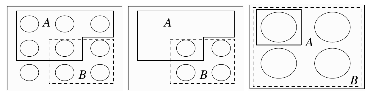
Three panels show a sample space of pebbles, removal of outcomes outside event B, and rescaling of the remaining probability masses to total one. — Conditioning removes outcomes incompatible with the evidence and renormalizes the remaining masses. Reproduced from Joseph K. Blitzstein and Jessica Hwang, *Introduction to Probability*, Figure 2.1, p. 44.

In the equal-mass version of the diagram, $B$ contains four of the nine pebbles and $A\cap B$ contains one. Before conditioning, $P(A\cap B)=1/9$ and $P(B)=4/9$. After conditioning:

\[P(A\mid B)=\frac{1/9}{4/9}=\frac14.\]

With unequal outcome probabilities, sum the masses instead of simply counting pebbles. Conditioning preserves the relative probabilities of the surviving outcomes.

Supplementary example: A die result known to be even

Roll a fair die. Let $A=\{4,5,6\}$ and $B=\{2,4,6\}$. Then:

\[P(A\mid B)=\frac{P(\{4,6\})}{P(\{2,4,6\})} =\frac{2/6}{3/6}=\frac23.\]

Originally, $P(A)=1/2$. The evidence changes the relevant possibilities to $2,4,6$, of which two satisfy $A$.

Core idea: Conditional probability changes the denominator to the probability of the evidence, not to the probability of the event being investigated.

The condition $P(B)>0$ is essential. The elementary ratio does not define $P(A\mid B)$ when $P(B)=0$. Conditioning on probability-zero information requires additional machinery beyond this definition.

The conditioning bar is not a set operation. $P(A\mid B)$ is a probability under specified information; it does not refer to an event called “$A\mid B$.”

Part 5 — Properties of conditional probability

For fixed $B$ with $P(B)>0$, define $Q(A)=P(A\mid B)$. This is itself a probability function:

\[Q(S)=\frac{P(S\cap B)}{P(B)}=1,\qquad Q(\varnothing)=0.\]

If $A_1,A_2,\ldots$ are disjoint, their intersections with $B$ are disjoint, so:

\[Q\left(\bigcup_i A_i\right) =\frac{\sum_i P(A_i\cap B)}{P(B)} =\sum_i Q(A_i).\]

Consequently, ordinary probability rules apply while keeping the evidence fixed. In particular:

\[P(A^c\mid B)=1-P(A\mid B),\] \[P(A\cup C\mid B)=P(A\mid B)+P(C\mid B)-P(A\cap C\mid B).\]

Also, $P(B\mid B)=1$, and $P(A\mid B)=1$ whenever $B\subseteq A$.

Independence as “no update”

For $P(B)>0$:

\[A\text{ and }B\text{ independent} \quad\Longleftrightarrow\quad P(A\mid B)=P(A).\]

Indeed, substituting $P(A\cap B)=P(A)P(B)$ into the definition cancels $P(B)$. Conversely, multiply the no-update equation by $P(B)$ to recover independence.

If $P(A)>0$ as well, independence also gives $P(B\mid A)=P(B)$. The product definition remains valid even when a conditional ratio would be undefined.

Part 6 — The multiplication rule for probabilities

Rearranging the conditional-probability definition gives:

\[\boxed{P(A\cap B)=P(B)P(A\mid B),\qquad P(B)>0.}\]

If $P(A)>0$, we can also write:

\[P(A\cap B)=P(A)P(B\mid A).\]

These are general multiplication rules. Independence allows the conditional factor to be replaced by its unconditional probability; without independence, the conditional factor must remain.

Supplementary worked example: Two hearts without replacement

Draw two cards in order from a uniformly shuffled standard deck. Let $H_1$ and $H_2$ denote a heart on the first and second draws.

The first draw is a heart with probability $13/52$. Given a first heart, twelve hearts remain among 51 cards:

\[P(H_1\cap H_2)=P(H_1)P(H_2\mid H_1) =\frac{13}{52}\frac{12}{51}=\frac1{17}.\]

The unconditional probability of a heart on the second draw is still $13/52=1/4$ by symmetry. But $12/51\ne1/4$, so the two heart events are dependent.

With replacement and independent draws, the second factor would be $13/52$, giving $1/16$ instead.

Core idea: The first result changes the composition of the remaining deck. The multiplication rule accounts for that change through a conditional probability.

Supplementary extension: Three events

Repeated application gives:

\[P(A\cap B\cap C)=P(A)P(B\mid A)P(C\mid A\cap B),\]

provided $P(A)>0$ and $P(A\cap B)>0$. The left-hand side is unchanged by reordering the events, but the conditioning events on the right must change with the chosen order.

Part 7 — Bayes’ rule: reversing the direction of conditioning

When $P(A)>0$ and $P(B)>0$, the two multiplication rules describe the same intersection:

\[P(A\mid B)P(B)=P(A\cap B)=P(B\mid A)P(A).\]

Divide by $P(B)$:

\[\boxed{P(A\mid B)=\frac{P(B\mid A)P(A)}{P(B)}.}\]

Bayes’ rule is useful when the conditional probability in one direction is easier to calculate than the one in the other direction.

For a hypothesis $H$ and evidence $E$:

\[P(H\mid E)=\frac{P(E\mid H)P(H)}{P(E)}.\]

Quantity	Interpretation
Prior, $P(H)$	Probability assigned before incorporating evidence $E$
Likelihood, $P(E\mid H)$	Probability of observing the evidence if $H$ holds
Evidence probability, $P(E)$	Overall probability of observing $E$
Posterior, $P(H\mid E)$	Updated probability after incorporating $E$

A high likelihood does not by itself imply a high posterior. The prior and the overall probability of the evidence also matter.

Incorrect: $P(A\mid B)=P(B\mid A)$ because both concern $A$ and $B$ occurring.

Correction: Both use the same numerator $P(A\cap B)$, but divide by different probabilities. In general:

\[P(A\mid B)=\frac{P(A\cap B)}{P(B)},\qquad P(B\mid A)=\frac{P(A\cap B)}{P(A)}.\]

Supplementary worked example: A heart first, given a red card second

Draw two cards without replacement. Let $A$ mean the first card is a heart, and $B$ mean the second card is red.

Find the easier direction: Given a first heart, 25 red cards remain among 51 cards:

\[P(B\mid A)=\frac{25}{51}.\]

Find the unconditional probabilities: The first card is a heart with probability $1/4$. Before either draw is observed, the second card is equally likely to be any of the 52 cards, so $P(B)=1/2$.

Reverse the conditioning:

\[P(A\mid B)=\frac{(25/51)(1/4)}{1/2}=\frac{25}{102}.\]

The two directions differ: $25/102$ versus $25/51$. As a check, their common intersection probability is:

\[P(A\cap B)=\frac14\frac{25}{51}=\frac{25}{204}.\]

Core idea: Information about the second draw can update the probability of the first. Conditioning concerns information, not a causal influence traveling backward in time.

Part 8 — Supplementary example: The exact evidence matters

Consider a family with two children. Use an idealized model in which each child is independently a girl or a boy with equal probability. List the elder child first, so the four equally likely outcomes are:

\[S=\{GG,GB,BG,BB\}.\]

Let $F$ be the event that both children are girls.

Evidence 1: At least one child is a girl

Let $E=\{GG,GB,BG\}$. Then $F\cap E=F$, and:

\[P(F\mid E)=\frac{1/4}{3/4}=\frac13.\]

The surviving family types are three equally likely outcomes, one of which is $GG$.

Evidence 2: The elder child is a girl

Let $E_1=\{GG,GB\}$. Then:

\[P(F\mid E_1)=\frac{1/4}{1/2}=\frac12.\]

Here the evidence designates a particular child, leaving two equally likely possibilities for the younger child.

Core idea: Both descriptions guarantee a girl, but they define different events. Conditional probabilities depend on the precise information and how it was obtained. Observing a randomly selected child is another experiment; it should not automatically be treated as conditioning on “at least one girl.”

Part 9 — Original practice questions

Try these before reading the answers.

Roll a fair die. Let $A=\{1,2\}$ and $B=\{3,4\}$. Are the events disjoint? Are they independent?
Suppose $A$ and $B$ are independent, with $P(A)=0.30$ and $P(B)=0.40$. Find $P(A\cap B^c)$, $P(A^c\cap B^c)$, and $P(A\cup B)$.
In the two-coin example with $A$ meaning first heads, $B$ second heads, and $C$ agreement, verify pairwise independence and explain the failure of mutual independence.
Roll four independent fair dice. Find the probability of exactly two sixes and the probability of at least two sixes.
In the Newton–Pepys twelve-dice game, explain why the complement includes exactly one six and why its count is $12\cdot5^{11}$.
Suppose $P(A)=0.40$, $P(B)=0.50$, and $P(A\cap B)=0.10$. Find $P(A\mid B)$, $P(B\mid A)$, and $P(A^c\mid B)$. Are the events independent?
Draw two cards without replacement. Find the probability of two aces. Compare with independent draws with replacement.
Suppose $P(H)=0.20$, $P(E\mid H)=0.60$, and $P(E)=0.30$. Find $P(H\mid E)$ and $P(H\cap E)$.
Under the idealized two-child model, compare the probability of two boys given at least one boy with the probability of two boys given that the younger child is a boy.

Part 10 — Practice answers

1. Disjoint die events

Their intersection is empty, so they are disjoint. But:

\[P(A\cap B)=0\ne\frac26\frac26=\frac19.\]

They are not independent. Learning that $A$ occurred rules out $B$.

2. Independent events and complements

Independence also holds for complements:

\[P(A\cap B^c)=0.30(0.60)=0.18,\] \[P(A^c\cap B^c)=0.70(0.60)=0.42.\]

The union probability is:

\[P(A\cup B)=0.30+0.40-0.30(0.40)=0.58.\]

It also equals $1-0.42$, by taking the complement of neither event occurring.

3. Pairwise but not mutual independence

All three events have probability $1/2$. Each pairwise intersection is $\{HH\}$, so its probability is $1/4=(1/2)(1/2)$.

The triple intersection is also $\{HH\}$, with probability $1/4$, rather than $1/8$. Thus the pairwise checks pass but the triple condition fails.

4. Four dice

Exactly two sixes:

\[P(\text{exactly two})=\frac{\binom42 5^2}{6^4} =\frac{150}{1296}=\frac{25}{216}\approx0.115741.\]

For at least two, subtract the disjoint zero-six and one-six cases:

\[P(\text{at least two})=1-\frac{5^4+4\cdot5^3}{6^4} =\frac{171}{1296}=\frac{19}{144}\approx0.131944.\]

5. The twelve-dice complement

Failing to obtain at least two sixes means obtaining either zero or one. For exactly one, choose its position in twelve ways. Each of the other eleven dice has five allowed non-six results, giving $12\cdot5^{11}$ outcomes. The two complement cases are disjoint, so their counts add.

6. Conditional probabilities

\[P(A\mid B)=\frac{0.10}{0.50}=0.20,\qquad P(B\mid A)=\frac{0.10}{0.40}=0.25.\]

Keeping the evidence $B$ fixed:

\[P(A^c\mid B)=1-0.20=0.80.\]

The events are dependent, since $P(A)P(B)=0.20\ne0.10=P(A\cap B)$.

7. Two aces

Without replacement:

\[P(\text{two aces})=\frac4{52}\frac3{51}=\frac1{221}\approx0.004525.\]

With replacement and independent draws:

\[P(\text{two aces})=\left(\frac4{52}\right)^2=\frac1{169}\approx0.005917.\]

Removing a first ace decreases the proportion of aces available for the second draw.

8. Bayesian update

\[P(H\mid E)=\frac{P(E\mid H)P(H)}{P(E)} =\frac{0.60(0.20)}{0.30}=0.40.\]

The joint probability is $P(H\cap E)=0.20(0.60)=0.12$. The likelihood $0.60$ and the posterior $0.40$ answer different questions.

9. Two kinds of evidence

Given at least one boy, the surviving outcomes are $BB,BG,GB$, each equally likely. Thus the probability of two boys is $1/3$.

Given that the younger child is a boy, only $BB,GB$ remain. The probability of two boys is $1/2$. The difference comes from conditioning on different events.

Part 11 — Quick revision sheet

Concept	Essential fact
Independence	$P(A\cap B)=P(A)P(B)$
Disjointness	$A\cap B=\varnothing$; disjoint positive-probability events are dependent
Complements of independent events	Complementing either or both preserves independence
Mutual independence	The intersection product rule must hold for every subset of events
Exactly $r$ sixes in $n$ fair independent rolls	$\binom nr5^{n-r}/6^n$
Newton–Pepys ranking	One six in six rolls is more likely than two in twelve or three in eighteen
Conditional probability	$P(A\mid B)=P(A\cap B)/P(B)$, with $P(B)>0$
Conditioning intuition	Remove outcomes outside the evidence, then renormalize
Conditional complement	$P(A^c\mid B)=1-P(A\mid B)$
Independence as no update	For $P(B)>0$, $P(A\mid B)=P(A)$
Multiplication rule	$P(A\cap B)=P(B)P(A\mid B)$
Bayes’ rule	$P(A\mid B)=P(B\mid A)P(A)/P(B)$
Direction of conditioning	$P(A\mid B)$ and $P(B\mid A)$ generally differ

Term Glossary

Independent events Definition

Events whose intersection probability equals the product of their individual probabilities. For positive-probability evidence, conditioning on one leaves the probability of the other unchanged.

Pairwise independence Definition

Independence of every pair in a collection of events. This does not guarantee independence of the collection as a whole.

Mutual independence Definition

The intersection product rule holding for every subset of two or more events in a collection.

Conditional probability Definition

A probability calculated with specified evidence treated as known, using the mass of the intersection divided by the mass of the evidence.

Renormalization Definition

Rescaling surviving probability masses so they total 1. When conditioning on $B$, each surviving mass is divided by $P(B)$.

Prior probability Definition

The probability of a hypothesis before incorporating the specified new evidence. It can already reflect other background information.

Likelihood Definition

The probability of the observed evidence given a hypothesis, $P(E\mid H)$. It is not the probability of the hypothesis given the evidence.

Posterior probability Definition

The updated probability of a hypothesis after conditioning on evidence, $P(H\mid E)$.

Bayes’ rule Theorem

A relation between the two directions of conditioning, obtained by writing the same intersection probability in two ways.

Statistics 110 Lecture 4 Independence Newton–Pepys Conditional probability Bayes’ rule

Lecture 5 - Conditioning Continued and the Law of Total Probability

Conditional probabilities depend on the exact evidence being used. The law of total probability combines simpler conditional calculations across disjoint cases, supplying the denominator needed in Bayes’ rule. Conditional independence allows multiplication within a specified context, but mixing contexts or selecting outcomes can create dependence that was absent within the original model.

Notation at a Glance

Symbol	Meaning
$P(A\mid B)$	Probability of $A$ given $B$, with $P(B)>0$
$A_1,\ldots,A_n$	A partition of $S$: disjoint cases covering the whole sample space
$P(B\mid A_i)P(A_i)$	Joint probability $P(B\cap A_i)$
$\sum_i P(B\mid A_i)P(A_i)$	Law of total probability for $P(B)$
$H_i$	One of several mutually exclusive, exhaustive hypotheses
$E$	Evidence being conditioned on
$P(A\mid B,E)$	Probability of $A$ given both $B$ and $E$; commas mean intersections
$D$, $T$	Disease and positive test result in a hypothetical test model
$P(T\mid D)$	Sensitivity: true-positive rate
$P(T^c\mid D^c)$	Specificity: true-negative rate
$P(A\cap B\mid E)=P(A\mid E)P(B\mid E)$	Conditional independence of $A$ and $B$ given $E$

Learning objectives

After studying these notes, you should be able to:

Distinguish “at least one ace,” “the ace of spades,” and “the first card is an ace” as different evidence.
Define a partition and derive the law of total probability from disjoint additivity.
Combine Bayes’ rule with a partition to calculate posterior probabilities.
Explain why a test’s sensitivity is different from the probability of a condition given a positive result.
Keep background conditioning consistent throughout a calculation.
Define conditional independence and distinguish it from unconditional independence.
Explain how an unknown shared factor or selected evidence can make two outcomes dependent.

Part 1 — Conditional examples: the exact evidence matters

Draw two cards without replacement from a uniformly shuffled standard deck. Let $F$ be the event that both cards are aces.

Because these questions concern the two-card hand rather than its draw order, use unordered hands as outcomes. There are:

\[\binom{52}{2}=1326\]

equally likely hands, of which $\binom42=6$ contain two aces.

Case 1: At least one card is an ace

Let $E$ be the event that the hand contains at least one ace. Count it using two disjoint cases:

Case	Count	Reason
Exactly one ace	$4\cdot48=192$	Choose one ace and one non-ace
Two aces	$\binom42=6$	Choose two of the four aces

Thus $\lvert E\rvert=198$. Since $F\subseteq E$:

\[\boxed{P(F\mid E)=\frac{6/1326}{198/1326}=\frac6{198}=\frac1{33}.}\]

An equivalent denominator is $\binom{52}{2}-\binom{48}{2}$, subtracting hands with no aces.

Case 2: The hand contains the ace of spades

Let $E_s$ mean that the ace of spades is one of the two cards. Fix that card and choose its companion from the other 51 cards. There are 51 such hands, and three have another ace:

\[\boxed{P(F\mid E_s)=\frac3{51}=\frac1{17}.}\]

The evidence identifies a particular card. The remaining card is uniformly distributed among the 51 other cards.

Case 3: The first card drawn is an ace

This evidence refers to draw order, so now use ordered outcomes. Given that the first card is an ace, three aces remain among 51 cards:

\[P(\text{two aces}\mid\text{first card is an ace})=\frac3{51}=\frac1{17}.\]

Cases 2 and 3 happen to give the same answer, but they are different conditioning events. Neither is equivalent to merely knowing that at least one card is an ace.

Incorrect: Knowing that there is an ace lets us remove it and treat the other card as uniform among 51 cards, giving $1/17$ in every case.

Correction: “At least one ace” does not designate which card was identified. Among its 198 compatible hands, only six contain two aces. The particular-card evidence and the at-least-one evidence select different collections of hands.

Core idea: A more specific conditioning event can change the probability of another event. The difference comes from the outcomes compatible with the evidence, not from the words “an ace” alone.

Part 2 — Partitions and the law of total probability

Partition Definition

Events $A_1,\ldots,A_n$ form a partition of $S$ if:

\[A_i\cap A_j=\varnothing\quad(i\ne j),\qquad \bigcup_{i=1}^{n}A_i=S.\]

Each outcome belongs to exactly one case. To use conditional probabilities $P(B\mid A_i)$, assume each case has positive probability.

For any event $B$, the pieces $B\cap A_i$ are disjoint and together cover $B$:

\[B=\bigcup_{i=1}^{n}(B\cap A_i).\]

By additivity and the multiplication rule:

\[P(B)=\sum_{i=1}^{n}P(B\cap A_i) =\sum_{i=1}^{n}P(B\mid A_i)P(A_i).\]

\[\boxed{P(B)=\sum_{i=1}^{n}P(B\mid A_i)P(A_i).}\]

This is the law of total probability, abbreviated LOTP.

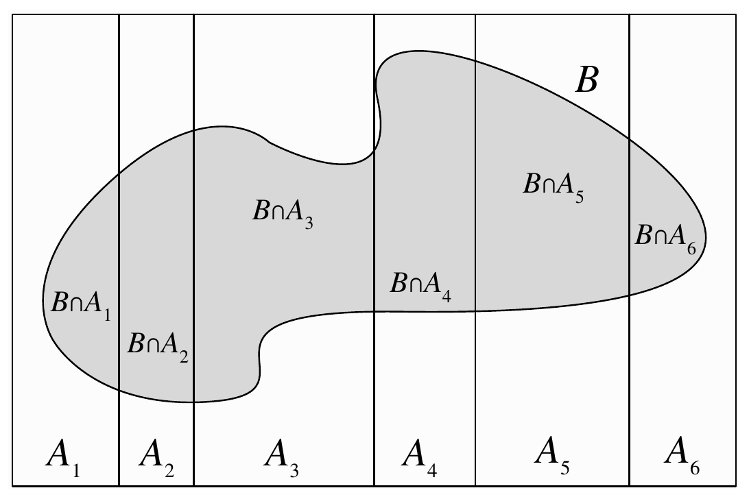
Sample space divided into six disjoint vertical cases; event B crosses the cases and is divided into pieces B intersection A one through B intersection A six. — A partition divides an event into disjoint contributions. Reproduced from Joseph K. Blitzstein and Jessica Hwang, *Introduction to Probability*, Figure 2.3, p. 50.

The weight $P(A_i)$ is the chance of being in case $i$; $P(B\mid A_i)$ is the chance of $B$ within that case. Their product is the contribution of that case to the overall probability.

Core idea: The unconditional probability is a weighted average of conditional probabilities. The weights sum to 1; they need not be equal.

Two complementary cases

For $0<P(A)<1$, the cases $A$ and $A^c$ form a partition:

\[\boxed{P(B)=P(B\mid A)P(A)+P(B\mid A^c)P(A^c).}\]

Disjoint and exhaustive are both required. Overlapping cases double-count some outcomes; cases that do not cover $S$ omit others. Adding $P(B\mid A_i)$ without multiplying by $P(A_i)$ also gives the wrong weighting.

If a case has probability zero, its joint contribution is zero. Omit it rather than treating an undefined conditional probability as a number to multiply by zero.

Part 3 — Bayes’ rule with a partition

Let $H_1,\ldots,H_n$ be a partition with positive prior probabilities, and suppose $P(E)>0$. Bayes’ rule gives:

\[P(H_j\mid E)=\frac{P(E\mid H_j)P(H_j)}{P(E)}.\]

Use LOTP to calculate the denominator:

\[\boxed{P(H_j\mid E)= \frac{P(E\mid H_j)P(H_j)} {\sum_{i=1}^{n}P(E\mid H_i)P(H_i)}.}\]

The numerator is the probability of hypothesis $j$ together with the evidence. The denominator is the total probability of that evidence across every possible hypothesis. Dividing assigns the fraction of the evidence probability attributable to hypothesis $j$.

Supplementary worked example: A randomly chosen coin

Choose once between a fair coin and a biased coin, each with probability $1/2$. The biased coin lands heads with probability $3/4$. Toss the selected coin three times, independently given which coin was selected, and observe $HHH$.

Let $F$ mean the coin is fair and $E$ mean three heads. The likelihoods are:

\[P(E\mid F)=\left(\frac12\right)^3=\frac18, \qquad P(E\mid F^c)=\left(\frac34\right)^3=\frac{27}{64}.\]

The total evidence probability is:

\[P(E)=\frac18\frac12+\frac{27}{64}\frac12 =\frac8{128}+\frac{27}{128}=\frac{35}{128}.\]

Hence:

\[\boxed{P(F\mid E)=\frac{(1/8)(1/2)}{35/128} =\frac8{35}\approx0.228571.}\]

The biased coin has posterior probability $27/35$. Three heads are possible under either coin, but are more likely under the biased coin, so the observation shifts probability toward that coin.

Core idea: Multiply within each hypothesis, add across the mutually exclusive hypotheses, and normalize to update their probabilities.

Incorrect: We observed $E$, so substitute $P(E)=1$ into Bayes’ rule.

Correction: Observing $E$ makes $P(E\mid E)=1$. The denominator $P(E)$ in Bayes’ rule is the probability of the evidence under the original model, before conditioning on it.

Part 4 — A test result: sensitivity, specificity, and the base rate

Consider a hypothetical test model. Let $D$ be the event that a person has a condition and $T$ the event of a positive result. Assume the person is drawn from a population with condition prevalence $p=P(D)$.

“95% accurate” is ambiguous unless the relevant conditional probabilities are stated. In this model, take:

\[P(T\mid D)=0.95,\qquad P(T^c\mid D^c)=0.95.\]

Thus the false-positive rate is $P(T\mid D^c)=0.05$. These are assumptions for an illustrative probability problem.

The desired probability after a positive result is $P(D\mid T)$, not $P(T\mid D)$. By Bayes’ rule and LOTP:

\[\boxed{P(D\mid T)= \frac{0.95p}{0.95p+0.05(1-p)}.}\]

The denominator includes both ways of getting a positive result: a true positive and a false positive.

Supplementary textbook example: Prevalence of 1%

For $p=0.01$:

\[P(T)=0.95(0.01)+0.05(0.99)=0.0095+0.0495=0.059,\] \[P(D\mid T)=\frac{0.0095}{0.059} =\frac{19}{118}\approx0.161017.\]

The probability rises from 1% before the result to about 16.10% afterward. The result is informative even though the posterior is much lower than the sensitivity.

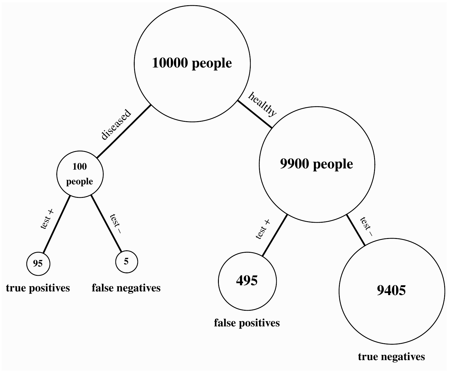
A model population of ten thousand divides into one hundred with the condition and nine thousand nine hundred without it, yielding ninety-five true positives and four hundred ninety-five false positives. — Expected counts in the hypothetical 1%-prevalence model, with 95% sensitivity and specificity. Reproduced from Blitzstein and Hwang, *Introduction to Probability*, Figure 2.4, p. 52. Bubble sizes are not to scale.

For 10,000 people under these proportions:

Group	Expected positive results	Expected negative results	Total
Condition present	95	5	100
Condition absent	495	9405	9900
Total	590	9410	10,000

Among positive results, the expected fraction with the condition is $95/590=19/118$. A small false-positive rate applied to a large condition-free group can produce more positives than a high true-positive rate applied to a small group.

Supplementary comparison: A rarer condition

Keeping the same test assumptions but changing the prevalence to $1/1000$ gives:

\[P(D\mid T)=\frac{0.95/1000}{0.95/1000+0.05(999/1000)} =\frac{19}{1018}\approx0.018664.\]

The sensitivity and specificity are unchanged, but the posterior is now about 1.87%. The prior prevalence affects the relative contributions of true and false positives.

Core idea: A conditional probability about how evidence is generated cannot be read directly as a probability about its underlying cause. The base rate supplies essential information.

The same reversal error in reasoning about evidence

A small probability of evidence given innocence, $P(E\mid I)$, does not equal a small probability of innocence given the evidence, $P(I\mid E)$. Bayes’ rule also requires the prior probabilities and the probability of the evidence under alternatives. Confusing these directions is called the prosecutor’s fallacy.

Part 5 — Keeping background conditioning consistent

For a fixed event $E$ with $P(E)>0$, the function $Q(B)=P(B\mid E)$ obeys the probability axioms. Consequently, LOTP and Bayes’ rule can be applied inside that conditional model.

Supplementary formula: LOTP with extra conditioning

For a partition $A_1,\ldots,A_n$, retaining positive-probability cases within $E$:

\[\boxed{P(B\mid E)=\sum_{i=1}^{n} P(B\mid A_i,E)P(A_i\mid E).}\]

The weights are now $P(A_i\mid E)$, not the original $P(A_i)$. The evidence can change the distribution of the cases themselves.

Supplementary formula: Bayes’ rule with extra conditioning

When $P(A\cap E)>0$ and $P(B\cap E)>0$:

\[\boxed{P(A\mid B,E)= \frac{P(B\mid A,E)P(A\mid E)}{P(B\mid E)}.}\]

The same background evidence $E$ appears in every probability. Commas to the right of the bar denote joint evidence, so $P(B\mid A,E)=P(B\mid A\cap E)$.

Core idea: Once a calculation is conditional on a context, both the case probabilities and within-case probabilities must use that context.

Part 6 — Conditional independence

Conditional independence Definition

For $P(E)>0$, events $A$ and $B$ are conditionally independent given $E$ if:

\[\boxed{P(A\cap B\mid E)=P(A\mid E)P(B\mid E).}\]

If also $P(B\cap E)>0$, this is equivalent to:

\[P(A\mid B,E)=P(A\mid E).\]

Given the context $E$, learning $B$ supplies no further information that changes the probability of $A$. This statement is about the probability model after conditioning, not necessarily about the original model.

Independence does not imply conditional independence. Conditional independence does not imply independence. Independence given $E$ also need not imply independence given $E^c$.

Supplementary example: An unknown shared coin creates dependence

Return to choosing once between the fair coin and the $3/4$-heads coin. Let $A$ and $B$ be heads on the first and second tosses.

Given the fair coin:

\[P(A\cap B\mid F)=\frac14=P(A\mid F)P(B\mid F).\]

Given the biased coin:

\[P(A\cap B\mid F^c)=\frac9{16}=P(A\mid F^c)P(B\mid F^c).\]

Thus the tosses are independent within each coin type. Without knowing the type:

\[P(A)=P(B)=\frac12\frac12+\frac34\frac12=\frac58,\] \[P(A\cap B)=\frac14\frac12+\frac9{16}\frac12=\frac{13}{32}.\]

But:

\[\frac{13}{32}=\frac{26}{64}\ne\frac{25}{64} =\left(\frac58\right)^2.\]

Indeed:

\[P(B\mid A)=\frac{13/32}{5/8}=\frac{13}{20}=0.65>\frac58.\]

A first head supplies evidence that the selected coin is biased, which in turn raises the probability of a second head.

Core idea: Multiplying within each known case is valid; averaging over an unknown shared case can introduce dependence. Choosing a fresh coin independently before every toss would describe a different experiment.

Example: Games against an opponent of unknown strength

Suppose repeated game results are independent once an opponent’s strength is known. If the opponent’s strength is unknown, an observed loss can make a strong opponent more plausible, changing the probability of losing the next game. Conditional independence within each strength category does not imply independence after those categories are mixed.

This is the same structure as the shared-coin example: one unknown factor affects several outcomes, and observing one outcome supplies information about that factor.

Part 7 — Conditioning can also create dependence

Supplementary worked example: At least one head

Toss two independent fair coins. Let $A$ mean first heads, $B$ mean second heads, and $E=A\cup B$ mean at least one head.

Before conditioning, $A$ and $B$ are independent. Given $E$, the three equally likely surviving outcomes are:

\[HH,\quad HT,\quad TH.\]

Therefore:

\[P(A\mid E)=P(B\mid E)=\frac23,\]

but:

\[P(A\cap B\mid E)=\frac13\ne\frac49 =P(A\mid E)P(B\mid E).\]

Once at least one head is known, learning that the first toss is tails forces the second to be heads:

\[P(B\mid A^c,E)=1.\]

The independent events have become dependent under the selected evidence.

Incorrect: Independence is a permanent property, so conditioning cannot change it.

Correction: Independence refers to a particular probability function. Conditioning changes that function. Always specify the context in which multiplication is justified.

Core idea: Restricting the sample space can remove combinations that originally made independence possible. Conditional independence must be checked using probabilities with the same evidence throughout.

Part 8 — Original practice questions

Try these before reading the answers.

Draw two cards without replacement. Find the probability of two kings given at least one king, and given that the king of hearts is in the hand.
Boxes A and B are chosen with probabilities $0.30$ and $0.70$. A draw is red with probability $0.80$ from A and $0.20$ from B. Find the overall red probability and the probability that a red draw came from A.
Explain why using “contains an ace” and “contains a heart” as the only two cases is not a valid partition of two-card hands.
Choose once between a fair coin and a $3/4$-heads coin, with equal probabilities, and observe two heads. Find the posterior probability that the coin is fair.
In a hypothetical population with prevalence $0.02$, a test has sensitivity $0.90$ and specificity $0.95$. Find the probability of a positive result and the posterior probability of the condition given a positive result.
For the preceding test model, find the probability of the condition given a negative result.
Suppose $P(A\mid E)=0.40$ and $P(B\mid E)=0.50$, with conditional independence given $E$. Find $P(A\cap B\mid E)$ and $P(A\cup B\mid E)$. Can you infer unconditional independence?
For the shared-coin example, compute $P(B\mid A)$ and compare it with $P(B)$. Explain what information the first head provides.
Toss two independent fair coins and condition on at least one head. Find the probability of second heads given first heads and the same evidence. Compare with the probability of second heads given only the at-least-one-head evidence.

Part 9 — Practice answers

1. Two kinds of king evidence

There are $4\cdot48+\binom42=198$ hands containing at least one king, of which six have two kings:

\[P(\text{two kings}\mid\text{at least one king})=\frac6{198}=\frac1{33}.\]

Given the king of hearts, its companion is one of 51 other cards, of which three are kings. The probability is $3/51=1/17$.

2. Mixture of boxes

By LOTP:

\[P(R)=0.80(0.30)+0.20(0.70)=0.38.\]

By Bayes’ rule:

\[P(A\mid R)=\frac{0.80(0.30)}{0.38}=\frac{12}{19}\approx0.631579.\]

The more red-heavy box becomes more likely after observing red.

3. Invalid cases

The events overlap: a hand may contain both an ace and a heart. They also fail to cover the sample space: a hand may contain neither. A valid partition could instead use the four combinations of containing or not containing an ace and containing or not containing a heart.

4. Two heads and coin identity

The likelihoods are $1/4$ and $9/16$. With equal priors:

\[P(F\mid HH)=\frac{(1/4)(1/2)}{(1/4)(1/2)+(9/16)(1/2)} =\frac4{13}\approx0.307692.\]

5. A positive test

The false-positive rate is $1-0.95=0.05$. Thus:

\[P(T)=0.90(0.02)+0.05(0.98)=0.067,\] \[P(D\mid T)=\frac{0.018}{0.067}=\frac{18}{67}\approx0.268657.\]

The posterior is about 26.87%, rather than the 90% sensitivity.

6. A negative test

The false-negative rate is $0.10$. Therefore:

\[P(T^c)=0.10(0.02)+0.95(0.98)=0.933,\] \[P(D\mid T^c)=\frac{0.10(0.02)}{0.933} =\frac2{933}\approx0.002144.\]

This is about 0.2144%. The positive and negative evidence probabilities sum to 1, but their corresponding condition posteriors do not have to do so: they condition on different events.

7. Conditional independence

\[P(A\cap B\mid E)=0.40(0.50)=0.20,\] \[P(A\cup B\mid E)=0.40+0.50-0.20=0.70.\]

These calculations apply within $E$. They do not determine whether $A$ and $B$ are independent without conditioning.

8. A shared unknown coin

\[P(B\mid A)=\frac{13/32}{5/8}=\frac{13}{20}=0.65, \qquad P(B)=\frac58=0.625.\]

The first head favors the biased coin, increasing the probability of heads on the second toss. The tosses are independent given coin type, but not after mixing the two types.

9. Selected coin outcomes

Given $A$ and $E$, only $HH$ and $HT$ survive, with equal probabilities, so:

\[P(B\mid A,E)=\frac12.\]

Given only $E$, the three outcomes $HH,HT,TH$ survive, giving $P(B\mid E)=2/3$. The difference shows that $A$ and $B$ are not conditionally independent given $E$.

Part 10 — Quick revision sheet

Concept	Essential fact
Exact evidence	At least one ace gives $1/33$ for two aces; a specified ace gives $1/17$
Partition	Pairwise disjoint cases whose union is $S$
LOTP	$P(B)=\sum_i P(B\mid A_i)P(A_i)$
Two-case LOTP	Split into $A$ and $A^c$, with both conditional probabilities defined
Partition form of Bayes	Posterior equals one likelihood-times-prior contribution divided by their total
Sensitivity	$P(T\mid D)$
Specificity	$P(T^c\mid D^c)$
False-positive rate	$P(T\mid D^c)=1-\text{specificity}$
Positive-result posterior	$P(D\mid T)$ depends on prevalence as well as test rates
Background evidence	Keep the same context to the right of the bar throughout a calculation
Conditional independence	$P(A\cap B\mid E)=P(A\mid E)P(B\mid E)$
Unknown shared factor	Independence within each case can become dependence after mixing cases
Selected evidence	Unconditional independence can disappear after conditioning

Term Glossary

Partition Definition

Disjoint events covering the whole sample space, so every outcome belongs to exactly one case.

Law of total probability Theorem

A formula combining within-case conditional probabilities with the probabilities of the cases to recover an overall probability.

Base rate Definition

The prior frequency or probability of a category before incorporating the specified new evidence. In the test model, it is condition prevalence.

Sensitivity Measure

The probability of a positive test result given that the condition is present, $P(T\mid D)$.

Specificity Measure

The probability of a negative test result given that the condition is absent, $P(T^c\mid D^c)$.

Prosecutor's fallacy Misconception

Confusing the probability of evidence under innocence with the probability of innocence given that evidence.

Conditional independence Definition

Independence under a specified conditional probability model. It does not establish independence outside that context.

Mixture Definition

A probability model formed by combining different case-specific models with weights given by their case probabilities.

Statistics 110 Lecture 5 Law of total probability Bayesian updates Conditional independence

Symbol	Meaning
\(S\)	Sample space: all possible outcomes
\(A\subseteq S\)	Event: a subset of the sample space
\(P(A)\)	Probability of event \(A\)
\(\lvert S\rvert\), \(\lvert A\rvert\)	Number of outcomes in the sample space and the event
\(n!\)	Factorial; \(0!=1\)
\(\binom nk\)	Number of unordered selections of \(k\) distinct objects from \(n\)
\(n\) and \(k\)	Number of available objects or types, and sample size
\(A\cup B\), \(A\cap B\), \(A^c\)	Union, intersection, and complement

Notation	Meaning
\(A\cup B\)	\(A\) or \(B\) occurs, including the possibility that both occur
\(A\cap B\)	Both \(A\) and \(B\) occur
\(A^c\)	\(A\) does not occur; the outcomes in \(S\) outside \(A\)
\(\varnothing\)	The empty event
\(A\subseteq B\)	Every outcome in \(A\) also belongs to \(B\)

Symbol	Meaning
\(n\)	Number of available types or labeled boxes in a stars-and-bars problem
\(k\)	Number of selections or identical objects to distribute
\(x_i\)	Number of selections of type \(i\), or occupancy of box \(i\)
\(\binom{n+k-1}{k}\)	Number of unordered selections with replacement
\(m,n\)	Sizes of two disjoint groups in Vandermonde’s identity
\(j\)	Number selected from the first group
\(S\)	Sample space
\(P(A)\)	Probability assigned to event \(A\)
\(\varnothing\)	Empty event
\(A_i\cap A_j=\varnothing\)	Events \(A_i\) and \(A_j\) are disjoint
\(\bigcup_{j=1}^{\infty}A_j\)	Event that at least one of the events \(A_1,A_2,\ldots\) occurs

Case	Direct reasoning	Formula check
\(k=0\)	One empty selection	\(\binom{n-1}{0}=1\)
\(k=1\)	Choose any one of the \(n\) types	\(\binom n1=n\)
\(n=1\)	Every selection is of the only type	\(\binom kk=1\)
\(n=2\)	The first count can be \(0,1,\ldots,k\); the second is determined	\(\binom{k+1}{k}=k+1\)

Number from the first group, \(j\)	Number from the second group	Number of committees
0	3	\(\binom30\binom43=4\)
1	2	\(\binom31\binom42=18\)
2	1	\(\binom32\binom41=12\)
3	0	\(\binom33\binom40=1\)

Event	Subset of the sample space
Both tosses are tails	\(\{TT\}\)
Exactly one head	\(\{HT,TH\}\)
At least one head	\(\{HH,HT,TH\}\)

Choice	Number of possibilities	Explanation
Rank of the three-card group	\(13\)	Any rank is possible
Three suits for that rank	\(\binom43=4\)	Choose three of its four cards
Rank of the two-card group	\(12\)	It must differ from the first rank
Two suits for that rank	\(\binom42=6\)	Choose two of its four cards

Sampling	Order matters	Order does not matter
With replacement	\(n^k\)	\(\binom{n+k-1}{k}\)
Without replacement	\(\frac{n!}{(n-k)!}\)	\(\binom nk\)

Concept	Essential fact
Sample space	Set of possible outcomes, \(S\)
Event	Subset \(A\subseteq S\)
Naive probability	\(P(A)=\lvert A\rvert/\lvert S\rvert\) for finite, equally likely outcomes
Multiplication rule	Multiply stage counts when each stage has the stated number of choices after every allowed history
Ordered, with replacement	\(n^k\)
Ordered, without replacement	\(n!/(n-k)!\)
Unordered, without replacement	\(\binom nk\)
Unordered, with replacement	\(\binom{n+k-1}{k}\)
Full house	\(13\binom43\cdot12\binom42/\binom{52}{5}\approx0.1441\%\)

Configuration	Ordered outcomes represented	Probability
Two heads	\(HH\)	\(1/4\)
One head and one tail	\(HT,TH\)	\(1/2\)
Two tails	\(TT\)	\(1/4\)

Method	First choice	Second choice	Total
President first	One of \(n\) people	Remaining \(k-1\) members from the other \(n-1\)	\(n\binom{n-1}{k-1}\)
Committee first	A \(k\)-person committee from \(n\)	President from its \(k\) members	\(\binom nk\,k\)

Counts \((x_A,x_B)\)	Number of ordered sequences	Probability
\((3,0)\)	1	\(1/8\)
\((2,1)\)	3	\(3/8\)
\((1,2)\)	3	\(3/8\)
\((0,3)\)	1	\(1/8\)

Symbol	Meaning
\(k\)	Number of people in the birthday problem
\(M\), \(M^c\)	At least one birthday match, and no birthday matches
\(\prod_{j=0}^{k-1}(1-j/365)\)	Product of the \(k\) factors for distinct birthdays
\(A^c\)	Complement of event \(A\) within \(S\)
\(B\cap A^c\)	Outcomes in \(B\) but outside \(A\)
\(A\subseteq B\)	Every outcome in \(A\) belongs to \(B\)
\(\bigcup_{i=1}^n A_i\)	At least one of the events \(A_1,\ldots,A_n\) occurs
\(\bigcap_{i\in I}A_i\)	All events whose indices belong to \(I\) occur
\(n\)	Number of distinct cards in the matching problem
\(\pi(i)\)	Label on the card in position \(i\) of a shuffled deck
\(A_i=\{\pi(i)=i\}\)	Card \(i\) matches its position
\(D_n\)	Number of permutations of \(n\) objects with no fixed points
\(e\)	Base of the natural logarithm; \(e\approx2.71828\)

People, \(k\)	Probability of at least one match
2	\(0.002740\)
10	\(0.116948\)
22	\(0.475695\)
23	\(0.507297\)
30	\(0.706316\)
50	\(0.970374\)
57	\(0.990122\)
100	\(0.999999693\)

Deck order	Matching positions	Result
\((1,2,3)\)	1, 2, 3	Win
\((1,3,2)\)	1	Win
\((2,1,3)\)	3	Win
\((2,3,1)\)	None	Lose
\((3,1,2)\)	None	Lose
\((3,2,1)\)	2	Win

Cards, \(n\)	Exact winning probability	Decimal
1	\(1\)	\(1.000000\)
2	\(1-1/2!\)	\(0.500000\)
3	\(1-1/2!+1/3!\)	\(0.666667\)
4	\(1-1/2!+1/3!-1/4!\)	\(0.625000\)
5	\(1-1/2!+1/3!-1/4!+1/5!\)	\(0.633333\)
6	\(1-1/2!+1/3!-1/4!+1/5!-1/6!\)	\(0.631944\)

Concept	Essential fact
Birthday sample space	\(365^k\) equally likely ordered assignments under uniformity and mutual independence
No birthday match	\(\prod_{j=0}^{k-1}(1-j/365)\) for \(1\le k\le365\)
At least one birthday match	One minus the no-match probability; exceeds 50% first at \(k=23\)
Guaranteed birthday match	\(k>365\)
Complement	\(P(A^c)=1-P(A)\)
Monotonicity	\(A\subseteq B\Rightarrow P(A)\le P(B)\)
Two-event addition	\(P(A\cup B)=P(A)+P(B)-P(A\cap B)\)
Inclusion–exclusion	Add singles, subtract pairs, add triples, and continue alternating
\(r\) specified card matches	\((n-r)!/n!\)
Total order-\(r\) contribution	\(\binom nr(n-r)!/n!=1/r!\)
Matching-game win	\(\sum_{r=1}^n(-1)^{r+1}/r!\)
Derangements	\(D_n=n!\sum_{r=0}^n(-1)^r/r!\)
Large-deck win probability	\(1-e^{-1}\approx0.632121\)

Symbol	Meaning
\(A\cap B\)	Both events \(A\) and \(B\) occur
\(P(A\mid B)\)	Probability of \(A\) given that \(B\) occurred; requires \(P(B)>0\)
\(P(A\cap B)=P(A)P(B)\)	Definition of independence of two events
\(A^c\)	Event that \(A\) does not occur
\(n\), \(r\)	Number of dice and number of sixes in a dice calculation
\(\binom nr\)	Number of choices of the \(r\) dice that show six
\(H\)	A hypothesis whose probability is being updated
\(E\)	Observed evidence
\(P(H)\)	Prior probability of the hypothesis
\(P(E\mid H)\)	Likelihood: probability of the evidence if the hypothesis holds
\(P(H\mid E)\)	Posterior probability after conditioning on the evidence

Game	Number of dice	Winning event
\(A\)	6	At least one six
\(B\)	12	At least two sixes
\(C\)	18	At least three sixes

Quantity	Interpretation
Prior, \(P(H)\)	Probability assigned before incorporating evidence \(E\)
Likelihood, \(P(E\mid H)\)	Probability of observing the evidence if \(H\) holds
Evidence probability, \(P(E)\)	Overall probability of observing \(E\)
Posterior, \(P(H\mid E)\)	Updated probability after incorporating \(E\)

Symbol	Meaning
\(P(A\mid B)\)	Probability of \(A\) given \(B\), with \(P(B)>0\)
\(A_1,\ldots,A_n\)	A partition of \(S\): disjoint cases covering the whole sample space
\(P(B\mid A_i)P(A_i)\)	Joint probability \(P(B\cap A_i)\)
\(\sum_i P(B\mid A_i)P(A_i)\)	Law of total probability for \(P(B)\)
\(H_i\)	One of several mutually exclusive, exhaustive hypotheses
\(E\)	Evidence being conditioned on
\(P(A\mid B,E)\)	Probability of \(A\) given both \(B\) and \(E\); commas mean intersections
\(D\), \(T\)	Disease and positive test result in a hypothetical test model
\(P(T\mid D)\)	Sensitivity: true-positive rate
\(P(T^c\mid D^c)\)	Specificity: true-negative rate
\(P(A\cap B\mid E)=P(A\mid E)P(B\mid E)\)	Conditional independence of \(A\) and \(B\) given \(E\)

Case	Count	Reason
Exactly one ace	\(4\cdot48=192\)	Choose one ace and one non-ace
Two aces	\(\binom42=6\)	Choose two of the four aces

Concept	Essential fact
Exact evidence	At least one ace gives \(1/33\) for two aces; a specified ace gives \(1/17\)
Partition	Pairwise disjoint cases whose union is \(S\)
LOTP	\(P(B)=\sum_i P(B\mid A_i)P(A_i)\)
Two-case LOTP	Split into \(A\) and \(A^c\), with both conditional probabilities defined
Partition form of Bayes	Posterior equals one likelihood-times-prior contribution divided by their total
Sensitivity	\(P(T\mid D)\)
Specificity	\(P(T^c\mid D^c)\)
False-positive rate	\(P(T\mid D^c)=1-\text{specificity}\)
Positive-result posterior	\(P(D\mid T)\) depends on prevalence as well as test rates
Background evidence	Keep the same context to the right of the bar throughout a calculation
Conditional independence	\(P(A\cap B\mid E)=P(A\mid E)P(B\mid E)\)
Unknown shared factor	Independence within each case can become dependence after mixing cases
Selected evidence	Unconditional independence can disappear after conditioning